01 · 基础：MHA → MQA → GQA → MLA¶

本篇是 sparse 与 linear 两条路线之前的基础。读这一篇之前，最好已经熟悉标准 scaled dot-product attention 的公式与 shape，并且知道 decode 阶段每生成一个 token 都要把整个 KV cache 从 HBM 读一遍——这一点在 Attention 机制第 1 节已经讲过。本篇沿用的统一记号见 Attention 机制 §2。

这一族机制有一个共同特点：不改 mask、不改递归，只改「一个 token 在 KV cache 里占多少个数」。所以整篇文章只有一条主线——每 token 每层的 KV cache 元素数，从 MHA 的 \(2 h d_h\) 一路压到 MLA 的 \(d_c + d_h^R\)。以 DeepSeek-V3 的量级为例，这个数字是从 32768 压到 576，相差 56.89 倍。

论文：MHA arXiv:1706.03762、MQA arXiv:1911.02150、GQA arXiv:2305.13245、MLA arXiv:2405.04434（DeepSeek-V2）与 arXiv:2412.19437（V3）。

1. MHA：定义与 KV cache 的来源¶

DeepSeek-V2 §2.1.1 的记法最适合往后衔接（\(h_t \in \mathbb{R}^d\) 是第 \(t\) 个 token 进 attention 前的 hidden state，\(n_h\) 个 head，每 head \(d_h\) 维）：

\[ q_t = W^Q h_t, \quad k_t = W^K h_t, \quad v_t = W^V h_t, \qquad W^{Q,K,V} \in \mathbb{R}^{d_h n_h \times d} \]

把 \(q_t, k_t, v_t\) 切成 \(n_h\) 份，得到 \(q_{t,i}, k_{t,i}, v_{t,i} \in \mathbb{R}^{d_h}\)，然后：

\[ \begin{aligned} o_{t,i} &= \sum_{j \le t} \mathrm{softmax}_j\!\left( q_{t,i}^{\top} k_{j,i} / \sqrt{d_h} \right) v_{j,i} \\ u_t &= W^O\, [o_{t,1}; \dots; o_{t,n_h}], & W^O &\in \mathbb{R}^{d \times d_h n_h} \end{aligned} \]

KV cache 从哪来：decode 第 \(t\) 步只算一个新 query，但 softmax 要遍历 \(j \le t\) 的全部 key/value。重算 \(k_{j,i}, v_{j,i}\) 需要重跑整个前缀，所以缓存它们。原文明确写 "MHA needs to cache 2 n_h d_h l elements for each token"（\(l\) = 层数）⇒

\[ \text{MHA}: \quad 2 n_h d_h \ \text{elements per token per layer} \]

这个数字有多严重，可以用一个例子说明：Llama-3-70B（\(n_h=64\)、\(d_h=128\)、80 层，实际用的是 GQA-8）如果换成纯 MHA，128K 上下文下的 KV cache 会是 2·64·128·80·131072·2B = 320 GiB，已经远超单卡容量。

2. MQA：只留一份 K/V¶

Shazeer 2019 §3 的原话是这样写的："Multi-query attention is identical except that the different heads share a single set of keys and values. The code … is identical to … multi-head attention, except that we remove the letter 'h' from the tf.einsum equations where it represents the 'heads' dimension of K, V, P_k, or P_v."

共享的是 K/V，Q 和 O 的投影仍然是 per-head：

tensor	MHA	MQA
\(P_q\)	\([h, d, k]\)	\([h, d, k]\)（不变）
\(P_k\)	\([h, d, k]\)	\([d, k]\)
\(P_v\)	\([h, d, v]\)	\([d, v]\)
\(P_o\)	\([h, d, v]\)	\([h, d, v]\)（不变）
logits einsum	`bhnk,bhmk->bhnm`	`bhnk,bmk->bhnm`
cache `prev_K`	\([b, h, m, k]\)	\([b, m, k]\)

arithmetic-intensity 分析¶

原文用三段分析给出了访存量 / 算术运算量的比值（\(m=n\)、\(k=v=d/h\)、\(n \le d\)）：

场景	算术运算	访存量	访存/算术
batched MHA（训练/prefill）	\(\Theta(bnd^2)\)	\(O(bnd + bhn^2 + d^2)\)	\(O(1/k + 1/(bn))\)
incremental MHA（decode，跨 \(n\) 步）	\(\Theta(bnd^2)\)	\(\Theta(bn^2d + nd^2)\)	\(\Theta(n/d + 1/b)\)
incremental MQA	\(\Theta(bnd^2)\)	\(\Theta(bnd + bn^2k + nd^2)\)	\(\Theta(1/d + n/(dh) + 1/b)\)

原文的论证链是这样展开的："When n ≈ d or b ≈ 1, the ratio is close to 1, causing memory bandwidth to be a major performance bottleneck… The 1/b term is the easier one — we can just use a larger batch size… Reducing the n/d term is harder. This term is related to the expense of reloading at each step the K and V tensors … which have size bhmk = bn²." 由此得到的结论是："We have reduced the offensive n/d by a factor of h."

这个论证背后的硬件前提原文也写明了："modern GPU/TPU hardware, where the computational capacity can be two orders of magnitude higher than the memory bandwidth."

这正是 Attention 机制 §1 那个式子最早的出处。\(n/d\) 项是 decode 阶段全部痛苦的根源，它正比于「每步要重新读的 KV cache 大小」除以「每步能做的算力」。可以说，整个基础机制这条线的历史，就是在不断压这一项。

代价：质量与稳定性¶

省下带宽不是没有代价的。Table 1（WMT14 EN-DE，211M 参数，为对齐参数量把 d_ff 从 4096 加宽到 5440）给出了质量对比：

Attention	`d_ff`	ln(PPL) dev	BLEU test (beam 1 / 4)
multi-head	4096	1.424	27.7 / 28.4
multi-query	5440	1.439	27.5 / 28.5
multi-head, \(h=1, d_k=128\)	6784	1.518	——
multi-head, \(h=2, d_k=64\)	6784	1.480	26.8 / 27.9
multi-head, \(h=8, d_k=16\)	6784	1.513	——

这里最值得记住的一点是：MQA 只掉了 0.015 的 ln-PPL，而「降低 head 数 \(h\)」或「降低每 head 维度 \(d_k\)」这两种替代性的省法却要掉 0.05–0.09，差了整整一个量级。换来的解码速度也很可观（TPUv2 μs/token）：MHA 是 1.7 + 46，MQA 是 1.5 + 3.8，decoder 部分快了 12 倍。

但还有一个更隐蔽的代价，写在 GQA 论文的 Appendix A 里，很多人读论文时会漏掉："multi-query attention can lead to training instability during fine-tuning, in particular combined with long input tasks… pre-training suffered from frequent loss spikes and the final models diverged immediately when fine-tuning on long-input tasks." 也就是说，MQA 在长输入任务上微调时可能直接训崩——这也是后面 GQA 要解决的问题之一。

3. GQA：分组共享与 mean-pool uptraining¶

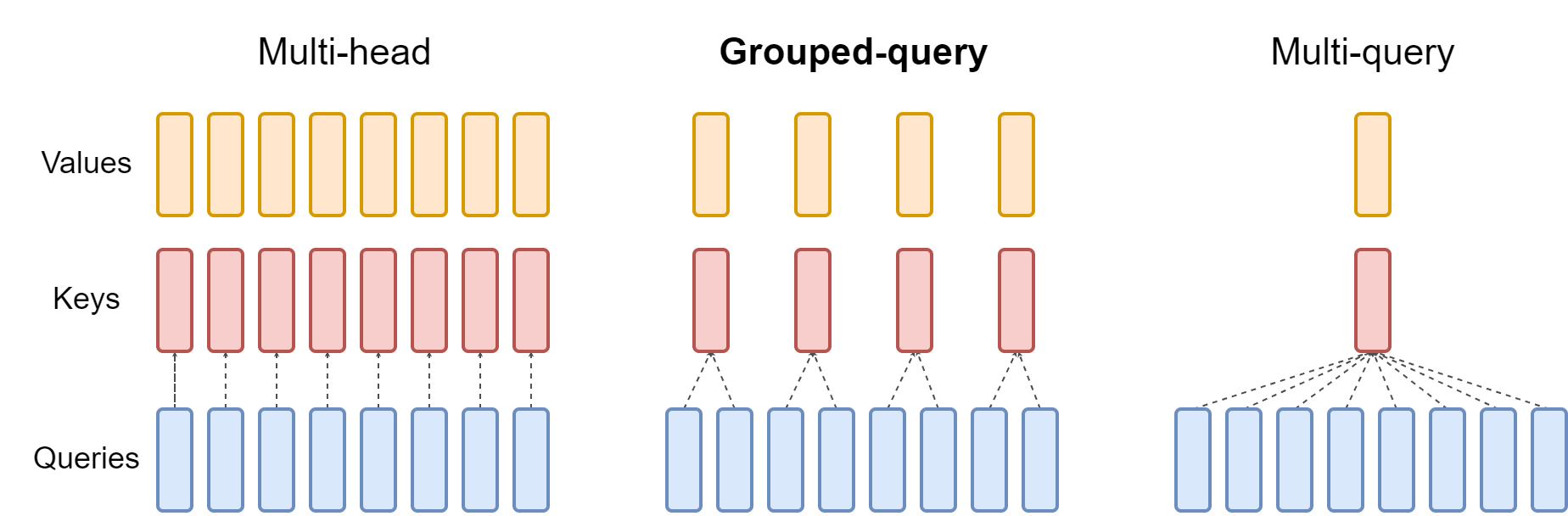
GQA：MHA（每个 query head 一份 KV）/ GQA（每组共享一份）/ MQA（全部共享一份）

图：GQA 论文的核心对照图（Ainslie et al. 2023, Fig 2；arXiv:2305.13245）。三种方案的唯一差别就是 KV head 的份数：MHA 留 \(h\) 份、GQA 留 \(g\) 份、MQA 只留 1 份。Q 的 head 数和 \(W^O\) 在三者中完全相同，这也正是为什么 GQA 可以从一个 MHA checkpoint「改造」而来，而不需要从头训练。

原文给出的定义是："Grouped-query attention divides query heads into G groups, each of which shares a single key head and value head. GQA-g refers to grouped-query with G groups. GQA-1 … is equivalent to MQA, while GQA-h … is equivalent to MHA."

三者其实可以用同一段代码表达，靠的是 repeat_interleave 把 \(h_{\mathrm{kv}}\) 份 KV 广播到 \(h\) 个 query head：

import math, torch

def gqa(q, k, v, causal=True):
    """q: [B, Hq, T, D];  k, v: [B, Hkv, T, D].  Hq % Hkv == 0.
    Hkv == Hq -> MHA;  Hkv == 1 -> MQA;  otherwise GQA-Hkv."""
    g = q.shape[1] // k.shape[1]
    k, v = k.repeat_interleave(g, dim=1), v.repeat_interleave(g, dim=1)
    s = q @ k.transpose(-1, -2) / math.sqrt(q.shape[-1])
    if causal:
        T = q.shape[-2]
        s = s.masked_fill(torch.ones(T, T, dtype=torch.bool, device=q.device).triu(1), float('-inf'))
    return s.softmax(-1) @ v

需要注意的是，repeat_interleave 会真的拷贝张量，而不是返回一个 view，所以在 kernel 外面这样写，相当于白白多读了 \(g\) 倍的 KV 带宽。真实的 kernel 用的是 pack_gqa：把共享同一个 KV head 的 \(g\) 个 Q head 打包进一次 KV 读取，让 KV 只从 HBM 读一次，具体见 04 · FA4（CuTeDSL）与工程接口 §5。这个「一个 KV entry 被多少 query 共享」的量，正是后面 NSA/DSA 设计的核心约束，会在 04 §5 再次出现。

Uptraining：把 MHA checkpoint 改造成 GQA¶

GQA 真正的工程贡献，其实不是这个架构本身，而是它不需要从头训练——已有的 MHA checkpoint 可以直接改造。做法分两步（原文逐字）：

Checkpoint conversion："The projection matrices for key and value heads are mean pooled into single projection matrices, which we find works better than selecting a single key and value head or randomly initializing new key and value heads from scratch." 对 GQA："we construct each group key and value head by mean-pooling all the original heads within that group."
继续预训练 \(\alpha\) 比例的原始训练步数（注意：是 steps / compute，不是 tokens）。

def mha_to_gqa(Wk, Wv, n_h, g):
    """Wk, Wv: [n_h * d_h, d].  返回 mean-pool 到 g 组后的投影。"""
    d = Wk.shape[-1]
    per = n_h // g                                    # 每组多少个原 head
    Wk_g = Wk.view(g, per, -1, d).mean(dim=1)          # 组内平均
    Wv_g = Wv.view(g, per, -1, d).mean(dim=1)
    return Wk_g.reshape(-1, d), Wv_g.reshape(-1, d)

具体数字上，\(\alpha = 0.05\) 大约需要 600 TPUv3 chip-days；论文写道"Both MQA and GQA gain from 5% uptraining with diminishing returns from 10%"，也就是超过 10% 之后收益就不明显了。消融实验里三种初始化方式的效果排序是 Mean > First > Random。

其中最重要的一句对比，也是决定了工业界为什么最终选 GQA 而不是 MQA 的关键：

"GQA already achieves reasonable performance after conversion while MQA requires uptraining to be useful." 以及 "Uptrained multi-query attention models are more stable but still display high variance… Uptrained grouped-query attention models, however, appear to be stable."

也就是说，GQA 转换完不训练也能用，MQA 必须靠 uptraining 才行；而且即使经过 uptraining，MQA 的稳定性还是不如 GQA。下面是 T5 上的结果（单位是 s/sample per TPUv4 chip）：

Model	`T_infer`	Average
MHA-Large	0.37	46.0
MHA-XXL	1.51	47.2
MQA-XXL (5% uptrained)	0.24	46.6
GQA-8-XXL (5% uptrained)	0.28	47.1

GQA 随模型规模变大的优势¶

论文给出了三条论据，说明为什么模型越大越适合 GQA，都值得记住。

第一条是关于压缩比例的："larger models generally scale the number of heads, such that multi-query attention represents a more aggressive cut in both memory bandwidth and capacity. GQA lets us keep the same proportional decrease … as model size increases." 也就是说，随着模型变大、head 数变多，MQA 相当于砍得越来越狠，而 GQA 可以保持固定的压缩比例。

第二条是关于带宽敞口的："larger models suffer relatively less from memory bandwidth overhead from attention, as the KV-cache scales with model dimension while model FLOPs and parameters scale with the square of model dimension." KV cache 只随模型维度线性增长，而 FLOPs 和参数量是平方增长，所以模型越大，attention 的带宽压力相对越轻。

第三条是 TP 场景下的工程理由，也是很多人容易忽略的一点："standard sharding for large models replicates the single key and value head by the number of model partitions; GQA removes the waste from such partitioning." 这里说的是 MQA 在张量并行（TP）下的隐藏成本：\(h_{\mathrm{kv}}=1\) 时每个 TP rank 都得存一份完整的 KV，而 \(h_{\mathrm{kv}} = \mathrm{TP}\) 时正好每个 rank 分到一份，不会有冗余。这也解释了为什么 \(g=8\) 这个配置出现得如此频繁（可以对照 02 · 整个 Transformer block 的切分方式里 attention 部分的切分方式）。

此外还有一条附带的说明：encoder 的 self-attention 不需要用 MQA/GQA 省带宽，因为"encoder representations are computed in parallel, and memory bandwidth is therefore generally not the primary bottleneck"——encoder 是并行计算的，带宽通常不是瓶颈。

论文选 8 组的理由写在 Fig 6 附近："Going from 1 (MQA) to 8 groups adds modest inference overhead, with increasing cost to adding more groups. We selected 8 groups as a favorable middle ground." 也就是从 1 组加到 8 组，推理开销增加得还算温和，再往上加代价就变大了，8 是一个折中点。

各模型的分组数 `g`¶

下表全部来自 HF 的 config.json，可以看到 \(g=8\) 确实是最常见的选择：

Model	hidden	layers	\(n_h\) (Q)	\(n_{\mathrm{kv}}\)（\(g\)）	\(d_h\)	Q:KV
Llama-3-70B	8192	80	64	8	128	8:1
Llama-3-8B	4096	32	32	8	128	4:1
Llama-4-Scout	5120	48	40	8	128	5:1
Mistral-7B-v0.1	4096	32	32	8	128	4:1
Qwen2.5-72B / Qwen3-32B	8192 / 5120	80 / 64	64	8	128	8:1
Qwen3-235B-A22B	4096	94	64	4	128	16:1
Qwen3-Next-80B-A3B	2048	48（12 attn）	16	2	256	8:1
Gemma-2/3-27B	4608 / 5376	46 / 62	32	16	128	2:1
gpt-oss-120b	2880	36	64	8	64	8:1
GLM-4.6	5120	92	96	8	128	12:1
MiniMax-M2	3072	62	48	8	128	6:1
OLMo-2-13B	5120	40	40	40	128	MHA

4. MLA：把 KV 压成一个 latent¶

前面 MHA→MQA→GQA 这条线，本质上都是在「留几份 K/V head」这一个维度上做取舍。MLA 换了一个维度来解决这个问题。

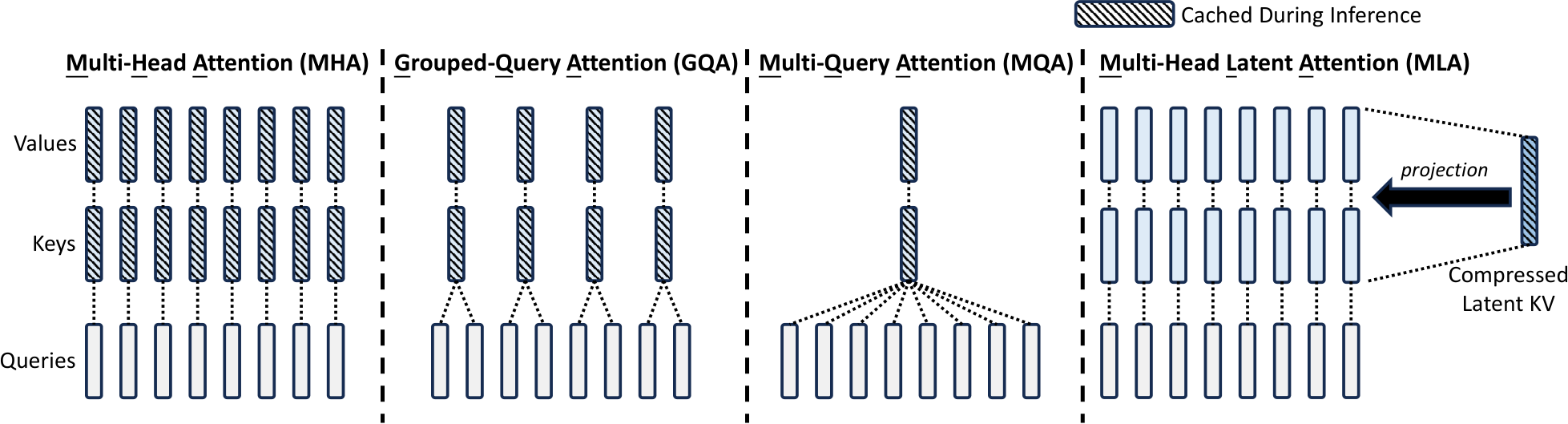
MHA / GQA / MQA / MLA 四联对比：MLA 只缓存一个压缩 latent c^KV，K/V 在推理时由它上投影还原（或被吸收掉）

图：DeepSeek-V2 的核心对照图（DeepSeek-AI 2024, Fig 3；arXiv:2405.04434）。MHA/GQA/MQA 都在「留几份 K/V head」这一个维度上做取舍，而 MLA 换了维度：缓存一个低秩 latent（图中橙色），K 和 V 都从它上投影得到。图右下角还标出了 decoupled RoPE 的那一小段 \(k^R\)，它是唯一另外需要缓存的东西。

MLA 的出发点是：GQA/MQA 都是在 head 维度上做硬性丢弃，但实际上 K/V 之间、head 之间存在大量冗余，不必靠丢弃来省空间，而是可以做低秩联合压缩。

4.1 KV 联合压缩（V2 Eq. 9–11）¶

\[ \begin{aligned} c_t^{KV} &= W^{DKV} h_t, & c_t^{KV} &\in \mathbb{R}^{d_c}, \quad d_c \ll d_h n_h \\ k_t^C &= W^{UK} c_t^{KV}, & W^{UK}, W^{UV} &\in \mathbb{R}^{d_h n_h \times d_c} \\ v_t^C &= W^{UV} c_t^{KV} \end{aligned} \]

其中 \(c_t^{KV}\) 是唯一需要缓存的主体。

4.2 Query 也做低秩（V2 Eq. 12–13）¶

\[ c_t^Q = W^{DQ} h_t, \quad c_t^Q \in \mathbb{R}^{d_c'}, \qquad q_t^C = W^{UQ} c_t^Q \]

原文点明了这样做的动机，这句话很容易被误读成「省 KV cache」，需要格外留意：

"in order to reduce the activation memory during training, we also perform low-rank compression for the queries, even if it cannot reduce the KV cache."

原因很简单：query 本来就不进 cache（decode 每步只算一个新 query），所以压缩它跟 KV cache 无关，纯粹是为了省训练期的 activation 内存。

4.3 Decoupled RoPE¶

这是 MLA 设计里唯一不那么优雅的部分，也是最值得花时间理解的部分。 原文（§2.1.3）是这样解释的：

"RoPE is position-sensitive for both keys and queries. If we apply RoPE for the keys k_t^C, W^UK in Equation 10 will be coupled with a position-sensitive RoPE matrix. In this way, W^UK cannot be absorbed into W^Q any more during inference, since a RoPE matrix related to the currently generating token will lie between W^Q and W^UK and matrix multiplication does not obey a commutative law. As a result, we must recompute the keys for all the prefix tokens during inference."

用代数说清楚。无 RoPE 时打分是：

\[ (W^{UQ}_i c_t^Q)^{\top} (W^{UK}_i c_j^{KV}) = c_t^{Q\top} \underbrace{(W^{UQ}_i)^{\top} W^{UK}_i}_{\text{indep. of } t,\, j}\, c_j^{KV} \]

中间那坨是常量矩阵，可以离线乘好——于是 \(c_j^{KV}\) 直接充当 key，\(W^{UK}\) 根本不用在推理时出现。加了 RoPE 之后：

\[ (R_t W^{UQ}_i c_t^Q)^{\top} (R_j W^{UK}_i c_j^{KV}) = c_t^{Q\top} (W^{UQ}_i)^{\top} \underbrace{R_{j-t}}_{\text{depends on } j-t}\, W^{UK}_i c_j^{KV} \]

问题就在这里：\(R_{j-t}\) 卡在两个投影中间，而它每一步都在变化，这意味着必须为每个前缀 token 现算 \(k_j^C\)，\(d_c\) 带来的压缩优势就全部作废了。

修法（V2 Eq. 14–19）：额外拉出一小段专门承载 RoPE，其中 query 侧 per-head、key 侧跨 head 共享（MQA 式）：

\[ \begin{aligned} \left[q_{t,1}^R; \dots; q_{t,n_h}^R\right] &= q_t^R = \mathrm{RoPE}(W^{QR} c_t^Q), & W^{QR} &\in \mathbb{R}^{d_h^R n_h \times d_c'} \\ k_t^R &= \mathrm{RoPE}(W^{KR} h_t), & W^{KR} &\in \mathbb{R}^{d_h^R \times d} \ \ \text{(no } i \text{ subscript)} \\ q_{t,i} &= [q_{t,i}^C ; q_{t,i}^R] \\ k_{t,i} &= [k_{t,i}^C ; k_t^R] & &\text{(shared } k^R \text{)} \\ o_{t,i} &= \sum_{j \le t} \mathrm{softmax}_j\!\left( q_{t,i}^{\top} k_{j,i} / \sqrt{d_h + d_h^R} \right) v_{j,i}^C \\ u_t &= W^O\, [o_{t,1}; \dots; o_{t,n_h}] \end{aligned} \]

这样一来，需要缓存的东西只剩两样：\(c_t^{KV}\)（\(d_c\) 维）加上 \(k_t^R\)（\(d_h^R\) 维）。

\[ \text{MLA}: \quad d_c + d_h^R \ \text{elements per token per layer} \]

注意这里没有因子 2——latent 同时充当 K 和 V。

这里 \(q^R\) 是 per-head 的，而 \(k^R\) 是单头共享的，这个不对称正是理解「MLA 吸收后就是 MQA」这句话的钥匙，§4.5 会展开讲。

4.4 矩阵吸收¶

Appendix C 结尾有一句话点出了矩阵吸收的原理："due to the associative law of matrix multiplication, we can absorb W^UK into W^UQ, and W^UV into W^O. Therefore, we do not need to compute keys and values out for each query." 也就是说，靠矩阵乘法的结合律，可以把两个投影矩阵吸收进别的矩阵里，从而避免每次都显式算出 key 和 value。本节把这个恒等式完整写出来，并用代码验证它。

拆开打分的两项：

\[ q_{t,i}^{\top} k_{j,i} = \underbrace{(q_{t,i}^C)^{\top} k_{j,i}^C}_{\text{NoPE, absorbable}} + \underbrace{(q_{t,i}^R)^{\top} k_j^R}_{\text{RoPE, shared } k^R} \]

吸收一（\(W^{UK}\) → query 侧）：

\[ (q_{t,i}^C)^{\top} k_{j,i}^C = (W^{UQ}_i c_t^Q)^{\top} (W^{UK}_i c_j^{KV}) = [\underbrace{(W^{UK}_i)^{\top} W^{UQ}_i c_t^Q}_{\tilde{q}_{t,i} \, \in \, \mathbb{R}^{d_c}}]^{\top} c_j^{KV} \]

这就推出了吸收一的结论：key 就是 latent 本身。

吸收二（\(W^{UV}\) → \(W^O\)）：

\[ u_t = \sum_i W^O_i\, o_{t,i} = \sum_i W^O_i W^{UV}_i \Big( \sum_j a_{t,j,i}\, c_j^{KV} \Big) = \sum_i \tilde{W}^O_i\, \tilde{o}_{t,i}, \qquad \tilde{W}^O_i = W^O_i W^{UV}_i, \quad \tilde{o}_{t,i} \in \mathbb{R}^{d_c} \]

同理，吸收二得到的结论是：value 也是 latent 本身。

这两条路径——直接还原 K/V 再算 attention，与吸收后直接用 latent 打分——理论上必须给出逐位相同的结果。下面这段代码把两条都实现出来并做对比，本篇所有数值都来自 float64 精度下的实测：

import math, torch

def mla_naive(h, W, pos):
    """MHA mode: 从 latent 还原 k^C / v^C，跑标准 MHA。训练 / prefill 用这条。"""
    T, nh, dh, dr = h.shape[0], W['nh'], W['dh'], W['dr']
    cQ, cKV = h @ W['Wdq'].T, h @ W['Wdkv'].T
    kR = rope(h @ W['Wkr'].T, pos)                                   # [T, dr]      共享
    qC = (cQ @ W['Wuq'].T).view(T, nh, dh)
    qR = rope((cQ @ W['Wqr'].T).view(T, nh, dr).transpose(0, 1), pos).transpose(0, 1)
    kC = (cKV @ W['Wuk'].T).view(T, nh, dh)                          # ← 物化出来
    vC = (cKV @ W['Wuv'].T).view(T, nh, dh)                          # ← 物化出来
    s = (torch.einsum('ihd,jhd->hij', qC, kC) +
         torch.einsum('ihr,jr->hij', qR, kR)) / math.sqrt(dh + dr)
    a = s.masked_fill(causal_mask(T), float('-inf')).softmax(-1)
    o = torch.einsum('hij,jhd->ihd', a, vC)
    return o.reshape(T, nh * dh) @ W['Wo'].T

def mla_absorbed(h, W, pos):
    """MQA mode: W^UK 吸进 query、W^UV 吸进 W^O。每个缓存 token 只读 c^KV 与 k^R。decode 用这条。"""
    T, nh, dh, dr, dc = h.shape[0], W['nh'], W['dh'], W['dr'], W['dc']
    cQ, cKV = h @ W['Wdq'].T, h @ W['Wdkv'].T
    kR = rope(h @ W['Wkr'].T, pos)
    qC = (cQ @ W['Wuq'].T).view(T, nh, dh)
    qR = rope((cQ @ W['Wqr'].T).view(T, nh, dr).transpose(0, 1), pos).transpose(0, 1)
    Wuk_h, Wuv_h = W['Wuk'].view(nh, dh, dc), W['Wuv'].view(nh, dh, dc)
    Wo_h = W['Wo'].view(-1, nh, dh)
    q_tilde = torch.einsum('ihd,hdc->ihc', qC, Wuk_h)                # 吸收一：q̃ ∈ ℝ^{d_c}
    s = (torch.einsum('ihc,jc->hij', q_tilde, cKV) +                 # key = latent 本身
         torch.einsum('ihr,jr->hij', qR, kR)) / math.sqrt(dh + dr)
    a = s.masked_fill(causal_mask(T), float('-inf')).softmax(-1)
    o_tilde = torch.einsum('hij,jc->ihc', a, cKV)                    # value = latent 本身
    Wo_tilde = torch.einsum('dhe,hec->dhc', Wo_h, Wuv_h)             # 吸收二
    return torch.einsum('ihc,dhc->id', o_tilde, Wo_tilde)

# 实测：rel_err(mla_absorbed, mla_naive) = 5.5e-16   ← 就是浮点噪声，两条路径数学上恒等

其中 rope 用论文 Eq. 34 的 interleaved 排布（\(x_{2i}\) 与 \(x_{2i+1}\) 配对）：

def rope(x, pos, base=10000.0):
    """x: [..., T, dr], dr 偶数。返回旋转后的 x。"""
    half = x.shape[-1] // 2
    freq = base ** (-torch.arange(half, dtype=x.dtype, device=x.device) / half)
    ang = pos[:, None].to(x.dtype) * freq[None, :]                   # [T, half]
    cos = ang.cos().repeat_interleave(2, -1)
    sin = ang.sin().repeat_interleave(2, -1)
    x_rot = torch.stack([-x[..., 1::2], x[..., 0::2]], dim=-1).flatten(-2)
    return x * cos + x_rot * sin

⚠️ HF 的 Llama 实现用的是 half-split 排布（\(x_i\) 配 \(x_{i + d_r/2}\)）。两者数学等价（只差一个维度置换），但权重不能混用。见 02 §2。

⚠️ 工程上不要真的把 \(\tilde{W} = (W^{UK}_i)^{\top} W^{UQ}_i\) 物化。DeepSeek-V3 每层 \(W^{UQ}\) 是 128·128×1536 = 25.2M、\(W^{UK}\) 是 128·128×512 = 8.4M，合计 33.6M；而 \(\tilde{W}\) 是 128×512×1536 = 100.7M，大了 3 倍。vLLM/SGLang 的做法是两次 GEMM：先 \(q^C_{t,i} = W^{UQ}_i c_t^Q\)，再 per-head bmm \(\tilde{q}_{t,i} = (W^{UK}_i)^{\top} q^C_{t,i}\)。

4.5 MHA mode 与 MQA mode¶

吸收之后，每个 query head 拿一个 \((d_c + d_h^R)\) 维 query，去和全体 head 共享的唯一一个 \((d_c + d_h^R)\) 维 key（就是 \([c_j^{KV} ; k_j^R]\)）打分，value 是共享的 \(d_c\) 维 \(c_j^{KV}\)——按定义这就是 MQA（\(n_{\mathrm{kv}} = 1\), \(d_{\mathrm{qk}} = 576\), \(d_v = 512\)）。

DeepSeek-V3.2 Appendix A 把这件事说成了一个显式的运行模式选择（Figure 7 caption 逐字）："For DeepSeek-V3.1-Terminus, the MHA mode is used for training and prefilling, while the MQA mode is used for decoding."

	MHA mode（unabsorbed）	MQA mode（absorbed）
用在	training / prefill（compute-bound）	decode（memory-bound）
做什么	从 \(c^{KV}\) 还原 \(k^C, v^C \in \mathbb{R}^{n_h d_h}\)，跑标准 FlashAttention	\(W^{UK}\) 吸进 query，\(W^{UV}\) 吸进 \(W^O\)
KV heads	\(n_h\) = 128	1
per-head QK 维	\(d_h + d_h^R\) = 192	\(d_c + d_h^R\) = 576
per-head V 维	\(d_h\) = 128	\(d_c\) = 512
每 token 每层需读的量	还原后 \(2 n_h d_h = 32768\) 元素	576 元素（56.9× 更少）

需要两种模式的原因是：prefill 时算力是瓶颈，MHA mode 的 per-head 维只有 192（对比 576），core-attention FLOPs 小 3.4 倍，而 KV 还原的上投影是一次性成本；decode 时带宽是瓶颈，MQA mode 只读 576 个数。同一组权重按阶段换算法，这是 MLA 设计上最精彩的地方。

4.6 具体数字与验算¶

V2 Table 1（原文逐字）：

Attention	KV Cache per Token (# Element)	Capability
MHA	\(2 n_h d_h l\)	Strong
GQA	\(2 n_g d_h l\)	Moderate
MQA	\(2 d_h l\)	Weak
MLA (Ours)	\((d_c + d_h^R)\, l \approx (9/2)\, d_h l\)	Stronger

caption："For DeepSeek-V2, d_c is set to 4 d_h and d_h^R is set to d_h/2. So, its KV cache is equal to GQA with only 2.25 groups, but its performance is stronger than MHA."

自己验算一遍（\(d_h = 128\)）：\(d_c = 512 = 4 d_h\) ✓，\(d_h^R = 64 = d_h/2\) ✓，\(d_c + d_h^R = 576 = 4.5\, d_h = (9/2)\, d_h\) ✓（这是精确相等而非近似——论文写 ≈ 只是因为 \(d_c = 4 d_h\) 是设计选择而非恒等式）。等效组数 \(2 n_g d_h = (9/2)\, d_h \Rightarrow n_g = 9/4 = 2.25\) ✓。MHA 与 MLA 的元素比为 \(32768/576 = 56.89\) ✓。

	DeepSeek-V2	DeepSeek-V3 / R1	Kimi K2
layers	60	61	61
\(d\)	5120	7168	7168
\(n_h\)	128	128	64
\(d_h\) (`qk_nope_head_dim`)	128	128	128
\(d_c\) (`kv_lora_rank`)	512	512	512
\(d_c'\) (`q_lora_rank`)	1536	1536	1536
\(d_h^R\) (`qk_rope_head_dim`)	64	64	64

⚠️ 三个易错点：其一，V2 是 \(d=5120\)、60 层，\(d=7168\)、61 层是 V3；其二，per-head QK 维是 192（128 维 NoPE 加 64 维 RoPE），而 V 是 128，所以 softmax scale 是 \(1/\sqrt{192}\) 而不是 \(1/\sqrt{128}\)；其三，训练稳定性需要额外的 norm——V2 §3.1.2："we employ additional RMS Norm layers after the compressed latent vectors, and multiply additional scaling factors at the width bottlenecks"。写 PyTorch 时别忘了 kv_a_layernorm 与 q_a_layernorm。

4.7 MLA 的质量对比¶

MLA 不只是更省，质量上确实优于 MHA。Appendix D.2 Table 9（MoE，同架构只换 attention）：

Benchmark	Small MoE + MHA	Small MoE + MLA	Large MoE + MHA	Large MoE + MLA
# Total Params	15.8B	15.7B	250.8B	247.4B
KV Cache/Token (#Elem)	110.6K	15.6K	860.2K	34.6K
BBH (3-shot)	37.9	39.0	46.6	50.7
MMLU (5-shot)	48.7	50.0	57.5	59.0
CMMLU (5-shot)	52.3	53.4	60.7	62.5

原文："MLA requires a significantly smaller amount of KV cache (14% for small MoE models and 4% for large MoE models) than MHA."（验算：15.6/110.6 = 14.1%、34.6/860.2 = 4.02% ✓）

配上 Appendix D.1 的 7B dense 对照（MQA 37.9 / GQA-8 41.2 / MHA 45.2 on MMLU），完整的结论链是：

质量：  MLA  >  MHA  >  GQA  >  MQA
cache： MLA(2.25 组)  ≪  GQA-8  <  MHA

MLA 在质量和 cache 两条轴上同时占优，这是它被 Kimi K2、Kimi Linear 等一路继承的原因。

摘要里的 "reduces the KV cache by 93.3%" 我复现不出来。按元素算（DeepSeek-67B 本身已是 GQA-8：2·8·128·95 = 243,200；V2 MLA：576·60 = 34,560）是减少 85.8%；最可能的解释是它按部署字节算，V2 §3.2.3 还做了「KV cache 量化到平均 6 bit」（34560·6/8 = 25,920 B vs 243200·2 = 486,400 B → 94.7%，接近但仍不精确）。文档里只引论文原话并给出元素级复现，不宣称能推出 93.3%。

5. GQA 到 MLA 的转换¶

既然 MLA 更好，能不能把已有的 GQA 模型改造过去？有两篇同期工作：

TransMLA（arXiv:2502.07864）：先证明「同等 KV cache 开销下 MLA 的表达力严格强于 GQA」，然后给出 training-free 转换。核心难点和 DeepSeek 自己遇到的一样——RoPE 阻断 Absorb。它用了两个技术：RoRoPE（对 key 输出做 PCA，把旋转跨 RoPE 两端施加，把所有 head 的主成分集中到第一个 head 的维度上；不变性条件是旋转矩阵只在所有 head 的同一维度内旋转、且 RoPE 实部虚部同样旋转）和 FreqFold（利用相邻 RoPE 维度频率相似来提升集中效率）。数字：LLaMA-2 压缩 68.75% 的 KV cache，6 个 benchmark 只掉 1.65%（training-free）；压 93% 再训 6B tokens 基本恢复；vLLM 上最高加速 10.6 倍。
MHA2MLA（arXiv:2502.14837）：partial-RoPE（按对 attention score 的贡献做 contribution-aware top-k 选维，把贡献小的维度的 RoPE 去掉）加 joint SVD（对 \(W_{k,\mathrm{nope}}\) 与 \(W_v\) 合并分解，SVD_joint 优于分别做的 SVD_split），只用 0.6%–1% 的训练数据。

partial-RoPE 这个想法后来被独立地大规模采用（Qwen3-Next 0.25、GLM-4.6 0.5、MiniMax 0.5、DeepSeek-V4 的 64 维），见 02 §3。

6. 小结¶

机制	每 token 每层元素	共享/压缩了什么	代价
MHA	\(2 n_h d_h\)	——	cache 巨大
MQA	\(2 d_h\)	全部 head 共享一份 K/V	质量掉、微调不稳定、TP 下要复制
GQA(\(g\))	\(2 g d_h\)	每 \(n_h / g\) 个 head 共享一份	可从 MHA mean-pool uptraining（5% steps），\(g=8\) 恰好对齐 TP
MLA	\(d_c + d_h^R\)	K/V 联合低秩压缩成一个 latent	需要 decoupled RoPE 这条「补丁」；prefill/decode 要跑两种模式
MLA + NoPE	\(d_c\)	连补丁都不要了	位置信息得由别人提供 → 见 `09`、`11`

最后一行是一个伏笔：Kimi Linear 让 MLA 层全部 NoPE，把位置编码的责任整个交给 KDA 层，于是 MLA 在推理时退化成纯 MQA，长上下文训练也不再需要 YaRN 调参。这是「基础」这条线和「linear」那条线的交汇点。

下一篇：02 · 位置编码与数值稳定 —— 位置编码和数值稳定看起来不是「attention 机制」，但 RoPE 能不能被吸收、NoPE 能不能用、logit 会不会失控，恰恰决定了上面每一个机制在真实模型里能否落地。