07 · 显存模型:总账、并行切分与配置演算¶
本篇是全章的总账篇:把单 rank 显存分成四大组成,每项给出可手算的公式(先定义每个符号),说清每种并行维切哪一块、batch 三个量各自动什么,最后在一组完整配置上演算到「离 80GB 还差多少」。机制细节一律不重复:recompute/offload 怎么做见 06,grad/param buffer 的结构见 05,ZeRO 账本的推导见 Data Parallelism(DP)、ZeRO 与 FSDP,PP in-flight 的调度分析见 03 · 显存、通信 overlap 与并行协同——本篇只算账。
阅读本篇需要的前置知识:
- 01 · 训练主循环 全篇,尤其 §3 的 batch 三量(
mbs/num_microbatches/ GBS)与 §8 的「常驻 vs 流动」引子(本篇是它的完整展开); - 四种并行维的切分直觉:TP 切层内矩阵、PP 切层、DP 切数据、CP 切序列(深入见 大规模训练的并行策略总览)。
代码锚点:theoretical_memory_usage.py(commit e03878b5f),即训练日志里 report_theoretical_memory 打印「theoretical memory footprints」的公式来源(training.py:L2698)。单位约定:全篇 GB = 10⁹ B;H100 标称 80GB = 80 GiB ≈ 85.9 GB,做预算时按 80 GB 保守估。注意源码打印的 "MB" 是 MiB(theoretical_memory_usage.py:L9)。
1. 显存的四大组成¶
单 rank 视角,先给出定义:
| 组成 | 内容 | 生灭节奏 |
|---|---|---|
| weights | 参与 forward/backward 计算的参数本体。bf16 训练下是 param buffer 里的 bf16 副本(DistOpt 时 param.data 被 remap 成 buffer 视图) |
常驻,跨 iteration 存活 |
| gradients | 连续 grad buffer(param.main_grad 所在),bf16 模型默认 fp32 累加(grad_reduce_in_fp32) |
常驻,每个 iteration 开头只清零不释放 |
| optimizer states | fp32 master weights + Adam m/v(DistOpt 下只持有 \(1/\mathrm{DP}\) 的 shard) |
常驻 |
| activations | forward 存给 backward 用的全部中间张量(含 dropout mask),峰值 = 单 micro-batch 量 × in-flight 份数 | 流动,随每个 micro-batch 生灭 |
| 其他 | logits & CE 中间量、通信 workspace(NCCL buffer / user buffer / RS-AG 暂存)、CUDA graph 内存池、对齐 padding、allocator 碎片 | 混合 |
前四类是「账面上的」,第五类是「实测总比公式多出来的那部分」(§8 专讲)。把 01 §8 那张「常驻 vs 流动」的图按四大组成重画一遍:
常驻(跨 iteration 存活,只清零不释放)——§2 的账
├── weights      param buffer(bf16)        2 B/param × P_shard
├── gradients    grad buffer(fp32 累加)     4 B/param × P_shard  ← 全量,不随 DP 缩
└── optimizer    fp32 master + m/v           12 B/param(DDP)或 12/DP(DistOpt)

流动(随每个 micro-batch 生灭)——§3 的账
├── activations  每层存给 backward 的张量      峰值 = 单层量 × 层数 × in-flight 份数
├── logits / CE  last stage 的 [b, s, V] 大图  ≈ 4·s·b·V/t(fp32),大 vocab 的刺客
└── 临时         param.grad 中转、通信 workspace、cuda graph 池、padding、碎片
省显存的所有手段,本质上都是在这张表的某一格上做文章:ZeRO 砍常驻的 optimizer 格,recompute/offload 砍流动的 activation 格,调小 mbs 线性缩 activation 格,TP/PP 把 \(P_{\text{shard}}\) 本身切小。
先看结论——§6 完整演算的结果(7B 级模型,TP=2/PP=2/DP=64,SP + selective recompute + DistOpt,first stage):
first stage 单 rank 峰值 ≈ 30 GB / 80 GB 预算
weights    (bf16 param buffer)    4.02 GB  ██
gradients  (fp32 grad buffer)     8.03 GB  ████
optimizer  (12 B/param ÷ DP=64)   0.38 GB  ▏
activations(SP + selective)      17.21 GB  ████████▌
其他 + 余量                      ~50 GB    ← fragment / workspace / 临时峰值都在这
每一条怎么算出来是 §2–§3 的内容;什么症状砍哪一条是 §4–§7 的内容。
2. 参数侧¶
2.1 每参数字节¶
定义:\(P_{\text{shard}}\) = 本 rank 持有的参数 element 数;\(\mathrm{DP}\) = data parallel size。单位:字节/参数。先把非 DistOpt 的 18 逐字节拆开(theoretical_memory_usage.py:L265–L268,源码注释明确假设「bf16 model params + fp32 main gradients + fp32 main params + fp32 Adam states」):
三种方案的账:
| 方案 | param (bf16) | grad (fp32 main grad) | fp32 master + m/v | 每参数字节 |
|---|---|---|---|---|
非 DistOpt(DDP / Float16OptimizerWithFloat16Params) |
2 | 4 | 4 + 8 | 18 |
DistOpt(ZeRO-1,use_distributed_optimizer) |
2 | 4 | \(12/\mathrm{DP}\) | \(6 + 12/\mathrm{DP}\) |
ZeRO-3 / FSDP(use_megatron_fsdp / torch FSDP) |
\(2/\mathrm{DP}\) | \(4/\mathrm{DP}\) | \(12/\mathrm{DP}\) | \(18/\mathrm{DP}\)(grad 若按 bf16 存则 \(16/\mathrm{DP}\),即论文 \(K=12\) 口径) |
两条必须记住的事:
- DistOpt 的 grad buffer 全量常驻、不随 DP 缩。
grad_data无条件按全量 \(P_{\text{shard}}\) 分配(param_and_grad_buffer.py:L1122–L1127),param_data在 DistOpt 下也是全量(:1113-1121);reduce-scatter 只是把结果写回本 rank 的 \(1/\mathrm{DP}\) 切片,buffer 本身一个字节没省。ZeRO-1 省的只有 optimizer 那 \(12\ \mathrm{B/param}\)(shard 区间甚至不尊重 param 边界,见05)。所以 DistOpt 下参数侧仍是「\(6\ \mathrm{B/param}\) 全量 \(+\ 12/\mathrm{DP}\)」,不是「\(18/\mathrm{DP}\)」。 - 18 的口径可变:
grad_reduce_in_fp32=False时 grad buffer 变 bf16,每参数 \(2\ \mathrm{B}\),非 DistOpt 就是 16 而非 18。fp16 训练另有 loss scale,但不改字节账。
ZeRO 频谱的完整推导与通信量守恒分析在 Data Parallelism(DP)、ZeRO 与 FSDP,这里只取结论图:
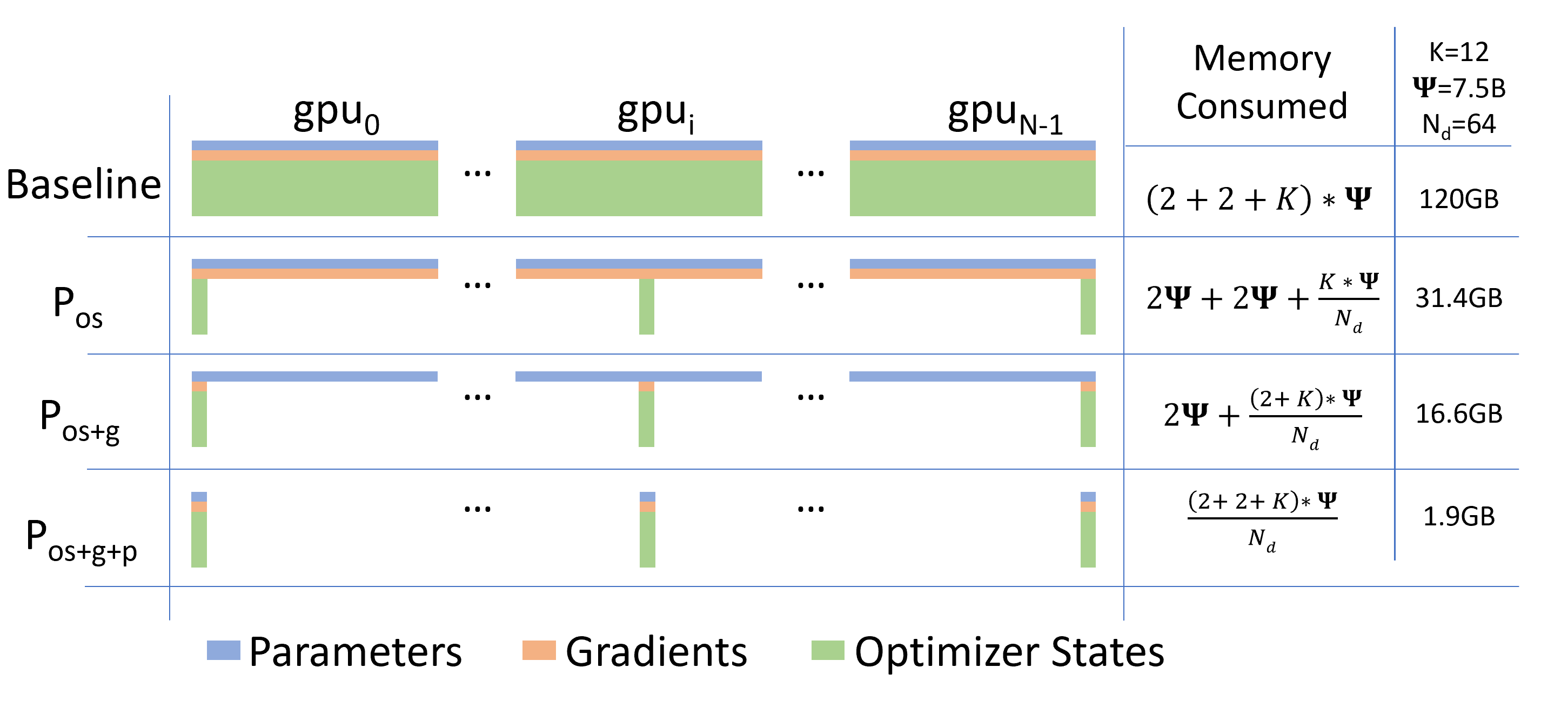
图:ZeRO 论文的显存账本图(
Ψ=参数量、K=optimizer state 系数,Adam 混精K=12、N_d=DP 度)。P_os(ZeRO-1,切 optimizer states)→P_os+g(ZeRO-2,再切 gradients)→P_os+g+p(ZeRO-3/FSDP,再切 parameters),每卡从16Ψ降到16Ψ/N_d。注意 Megatron DistOpt 对应P_os但工程上 grad buffer 仍全量常驻(上表第 2 行),这是实现选择与论文理想账的差异。(Rajbhandari et al. 2019, Fig 1;arXiv:1910.02054)
2.2 参数量估算¶
dense GPT 风格模型(GQA、SwiGLU、RMSNorm、embedding 与 output 共享权重),符号:\(h\)=hidden size,\(L\)=层数,\(a\)=attention head 数,\(g\)=GQA 的 kv head 数(num_query_groups),\(d\)=head dim(kv_channels),\(q = ad\)=query projection size,\(\mathit{ffn}\)=MLP intermediate size,\(V\)=padded vocab size:
P ≈ L · [ 2·h·q·(1 + g/a)  +  3·h·ffn  +  2·h ]  +  V·h
           └ attention ┘      └ SwiGLU ┘   └ 2 LN ┘   └ embedding(tied) ┘
- attention 项:\(W_q: h \times q\),\(W_k = W_v: h \times (gd)\),\(W_o: q \times h\)。MHA 特例(\(g=a\)、\(q=h\))退化成 \(4h^2\);GQA 时按 \(g/a\) 修正。对应源码
self_attn_term,即 \(2h^2(1 + g/a)(q/h)\)(theoretical_memory_usage.py:L82–L93;\(q/h\) 即query_projection_to_hidden_size_ratio,:14-15;非 GQA 时num_query_groups置为 \(a\),:17-18)。MLA 有单独分支(:62-80)。 - MLP 项:SwiGLU 三个矩阵(w1/w3 升维、w2 降维)对应 \(3h\,\mathit{ffn}\),源码写作 \(2h\,\mathit{ffn}\times\)
gated_linear_multiplier,swiglu时 multiplier = \(3/2\)(:21, :103);非 gated MLP 是 \(2h\,\mathit{ffn}\)。 - LN 项:每层两个 LN;RMSNorm 无 bias,
norm_size=1,即 \(2h\)(:60, :113)。另有 block 末尾的 final LN(:96, :147)。 - embedding 项:\(Vh\);
untie_embeddings_and_output_weights时乘 2(:97-100)。注意公式用的是 padded vocab size(:95)。 - MoE:按
moe_layer_freq把层拆成 dense/moe 两类(:29-50),moe 层的 MLP 项换成 \(2h \cdot \mathit{moe\_ffn} \cdot E \cdot \mathrm{multiplier}\)(\(E\) = expert 数,:105-107),再加 router \(hE\)(:114-118)与 shared expert(:104)。源码还算了num_active_parameters(只计 top-k 个 routed expert,:108-112, :136-143)——算 FLOPs 用 active、算显存用全量,两者不要混。
每 rank 的 \(P_{\text{shard}}\):源码按「最重 shard」估——首个 PP stage 持有 \(1/\mathrm{PP}\) 的层 + embedding(+ MTP block),TP 切分的部分除 \(\mathrm{TP}\),expert 部分除 \(\mathrm{ETP}\cdot\mathrm{EP}\),LayerNorm/router 等复制参数不除(:219-244):
这也是为什么首尾 stage 的参数侧显存比中间 stage 多一块 embedding——PP 各 stage 的 weights/grads/optimizer 并不均分。
3. activation¶
3.1 符号与基线公式¶
符号(与前节一致,新增):\(s\)=seq length,\(b\)=micro-batch size,\(t\)=TP size,\(p\)=PP size,\(v\)=VPP size,\(m\)=num_microbatches。activation 以 16-bit 存储(\(2\ \mathrm{B/elem}\)),dropout mask \(1\ \mathrm{B/elem}\)(论文 §4 的假设)。无任何并行时,每层要存的 activation(arXiv:2205.05198 eq.1):
逐项 breakdown(论文 §4.1,「存什么」取决于 backward 算梯度需要的输入):
| 部分 | 存的张量 | 字节 |
|---|---|---|
| attention | QKV 投影的输入 \(2sbh\);\(QK^{\top}\) 的 Q、K \(4sbh\);softmax 输出 \(2as^2b\);softmax dropout mask \(as^2b\);attention-over-V 的 dropout 输出 \(2as^2b\) 与 V \(2sbh\);output 投影输入 \(2sbh\);attention dropout mask \(sbh\) | \(11sbh + 5as^2b\) |
| MLP | fc1 输入 \(2sbh\);GeLU 输入 \(8sbh\);fc2 输入 \(8sbh\);dropout mask \(sbh\)(intermediate = \(4h\)) | \(19sbh\) |
| LayerNorm ×2 | 各存输入 \(2sbh\) | \(4sbh\) |
| 合计 | \(sbh(34 + 5as/h)\) |
关键观察:\(5as/h\) 这项随 \(s\) 线性增长,\(s\) 一长就远超 34。本配置(\(a=32, s=4096, h=4096\))下 \(5as/h = 160\),\(s^2\) 项是线性项的近 5 倍。这就是 selective recompute 的全部动机(§3.3)。
3.2 TP 与 SP 各切哪一部分¶
- 只有 TP:块内的矩阵乘法 activation 被切,但两个 LN、两处 dropout、两个块的输入在 TP 组内复制(它们不在 TP 的切分路径上)。每层(eq.2)为 \(M_{\mathrm{layer}}(\mathrm{TP}) = sbh\left(10 + \frac{24}{t} + \frac{5as}{ht}\right)\)。不除 \(t\) 的「10」= LN 输入 4 + 两个 dropout mask 2 + QKV/fc1 两个块输入各 2——TP 切不掉的部分。
- TP + SP:sequence parallelism 把 LN/dropout 区域沿 seq 维切开,于是所有项都能除 \(t\),每层(eq.4)为 \(M_{\mathrm{layer}}(\mathrm{TP+SP}) = \frac{sbh}{t}\left(34 + \frac{5as}{h}\right)\)。
SP 不增加通信量(ring all-reduce = reduce-scatter + all-gather,与 TP 的 all-reduce 同带宽),机制见 Tensor Parallelism(TP)与 Sequence Parallelism(SP)。
3.3 recompute 三档¶
| 档位 | 每层存储 | 总量(first stage,TP+SP) | 计算代价 |
|---|---|---|---|
| 不 recompute | \(sbh(34+5as/h)/t\) | eq.5:\((sbhL/t)(34+5as/h)\) | 0 |
| selective | 砍掉 \(5as^2b\)(\(QK^{\top}\)/softmax/dropout/attn-over-V 反向重算),保留全部线性项 | eq.6:\(34sbhL/t\) | FLOPs +2.7%(GPT-3)/ +1.6%(MT-NLG);实测 530B/1T 仅 ~2% step |
| full | 只存每层输入 \(2sbh\) | \(2sbhL\)(可再除 \(t\) 但要多一次 all-gather,论文不取) | +30–40% step time |
论文 Table 4(22B 单层实测):selective 的 fwd+bwd 开销 7%,full 是 39%;selective + SP 组合只剩 4%。机制(重算什么、RNG 怎么保证正确)见 06。
3.4 Megatron 的 compute_activation_memory¶
theoretical_memory_usage.py:L280–L351 把上面几步拼成「first stage 峰值」的完整公式(SP + selective 分支)。先给总定义式,再逐步对行号:
M_first_stage = [ s·b·h·(18 + 4·ffn/h)·L + 8·s·b·p + s·b·h·p ] · penalty · discount / t
                └──────── 层 ────────┘   └ embedding 两项 ┘
penalty  = 1 + (p-1)/(p·v)   (仅 VPP;:314-327)
discount = min(1, m/p)       (仅非 interleaved 且 m < p;:331-336)
p == 1 时再加 output 项 4·s·b·h·(1 + V/h)(:340-348,加在 ÷t 之前)
逐步对应:
① 每层每 micro-batch:  s·b·h·(18 + 4·ffn/h)                :289-291
② × L(= L/p 层 × p 个 in-flight micro-batch)              :297
③ + embedding 输入 8·s·b·p(token id,int64 8 B)           :302-304
  + embedding dropout mask s·b·h·p(1 B/elem)               :306-311
④ × VPP 惩罚 1 + (p-1)/(p·v)              (有 VPP 时)      :314-327
⑤ × min(1, m/p)      (非 interleaved 且 m < p 时打折)      :331-336
⑥ + output layer/CE 4·s·b·h·(1 + V/h)   (仅 p == 1)        :340-348
⑦ ÷ t                                                   :350-351
几处值得停顿:
- ① 与论文的对应:\(18 + 4\,\mathit{ffn}/h\) 就是 eq.6 的 34 把 MLP 的 \(4h\) 推广成任意 \(\mathit{ffn}\)——\(19sbh\)(MLP,\(\mathit{ffn}=4h\))\(= sbh(3 + 4\,\mathit{ffn}/h)\),加 attention 线性部分 11、LN 4,得 \(18 + 4\,\mathit{ffn}/h\)。\(\mathit{ffn}=4h\) 时精确等于 34。\(s^2\) 项消失就是 selective recompute 的效果(源码注释即声明用论文 Table 2,:281)。
- ② 为什么不除 \(p\):1F1B 下 first stage 必须在途 \(p\) 个 micro-batch 才能压住流水线(warmup 公式 \(\mathrm{num\_warmup} = \min(p - \mathrm{rank} - 1, m)\),
schedules.py:L2227;steady 段栈深 = warmup + 1,因此 first stage 峰值 \(p\) 份)。\(p\) 份乘 \(L/p\) 层等于 \(L\) 层的量——PP 对 first stage 的 activation 没有减免(论文 §4.2.3 的原话结论),PP 省的是 weights/optimizer。in-flight 的完整分析见 03 · 显存、通信 overlap 与并行协同。 - ③ 的两项为什么乘 \(p\) 不乘 \(L\):embedding 只在 first stage 出现一次,但它的输入与 dropout mask 要为每个在途 micro-batch 各存一份,所以按 \(p\) 份计。
- ④ VPP 惩罚:interleaved 调度每 rank 持有 \(v\) 个不连续 chunk,在途 micro-batch 变多,activation 乘 \(1 + (p-1)/(pv)\)(:314-327,即论文 eq.5 后那段「interleaving 要乘 \((1+(p-1)/(pm))\)」;注意论文符号 \(m\) 是 interleaving 的 stage 数,即本篇的 \(v\),与本篇符号表的 \(m\)=num_microbatches 不是一回事)。VPP 用显存换 bubble,代价就写在这里。
- ⑤ \(m < p\) 打折:非 interleaved 且 \(m < p\) 时,在途只有 \(m\) 份,乘 \(\min(1, m/p)\)(:331-336)。省显存是真,但此时流水线根本压不满,bubble 爆炸,正常配置不该落进这个分支。
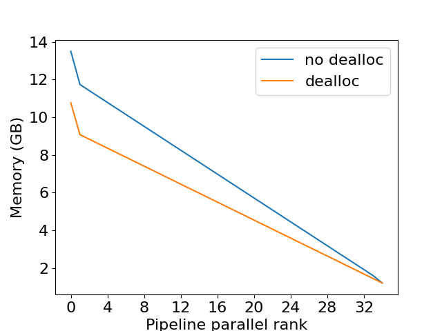
图:1F1B 各 PP stage 的峰值 activation——first stage 要存
p个在途 micro-batch,逐级递减到 last stage 的 1 个。这解释了为什么 first stage 最容易 OOM,也是本篇 §6 演算对 first stage 单独汇总的原因。(Korthikanti et al. 2022, Fig 9;arXiv:2205.05198)
3.5 logits 与 CE¶
⑥ 的 \(4sbh(1 + V/h)\) 只在 \(p = 1\) 时计入(:340-348)——因为整个函数估的是 first stage(:282-283 注释),而 logits/CE 物理上发生在 last stage(loss 只在 last stage 算,training.py:L2327)。所以 PP > 1 时这套公式对 last stage 少报了一块,演算时要自己补上。
这项的构成(论文 §4.3,与源码同口径):final LN 输入 \(2sbh\) + output 投影输入 \(2sbh\) + fp32 logits \(4sbV\),合计 \(4sbh(1 + V/h)\)。源码把它加在全局 \(\div t\) 之前(:350-351),即实际按 \(4sbh(1+V/h)/t\) 计——对应 vocab 维被 TP 切开、CE 前 fp32 upcast 的实现。
为什么这项需要单独警惕:它约等于 \(4sbV/t\),与 \(V\) 成正比且与层数无关——\(V\)=128k 时单 micro-batch 就是 GB 级(§6 算出 2.1 GB),\(V\) 再大或 \(b\) 一涨它先爆;而它只落在 last stage 一张卡上,监控里表现为「last stage 莫名比 middle stage 高几 GB」。大 vocab 模型(\(V\) ≥ 128k)务必把它单列进账。
3.6 compute_activation_memory_without_sp¶
report_theoretical_memory 只在 sequence_parallel and recompute_granularity == 'selective' 时走上面的 SP 公式,否则走 compute_activation_memory_without_sp(分支选择 :438-449):
- 每层 \(sbh(10 + 24/t)\)(:358)——正是 eq.2 去掉 \(s^2\) 项(隐含假设 fused/flash attention 不落地 \(s \times s\) 矩阵),且不显式建模 recompute;
- embedding 两项、VPP 惩罚、\(m<p\) 打折与 SP 版相同(:371-407);
- \(p = 1\) 时 output 项是 \(2(sbV/t + sbh)\)(:410-419,注意系数是 2 不是 4——只按 bf16 logits 计,与 SP 版口径不同);
- 末尾统一乘 1.05,给 optimizer/临时量留 overhead(:421-423)。
看训练日志里的 theoretical memory 数字前,先确认走的是哪个分支——两个公式的口径差异(\(s^2\) 项、output 系数、1.05)会让数字差出一大截。
4. 每种并行维切哪一块¶
| 并行维 | weights | grads | optimizer | activations | 主通信 | 备注 |
|---|---|---|---|---|---|---|
| TP(层内切矩阵) | 切:attention/MLP 矩阵 \(\div t\)(§2.2 的 attention/MLP 项) | 同 weights 切 | 同 | 块内切、LN/dropout 复制(eq.2 的「10」切不掉) | 每层 4× all-reduce(fwd 2 + bwd 2,attention/MLP 各一) | 通信量大,限机内 NVLink |
| SP(TP 的补充) | 不切 | 不切 | 不切 | LN/dropout 区沿 seq 维 \(\div t\) → 全部 \(\div t\)(eq.4) | RS + AG 对(带宽与 all-reduce 相同) | 必须与 TP 同开;selective 公式的前提 |
| PP(切层) | 切:\(\div p\)(按层分 stage) | 同 | 同 | 层 \(\div p\) 但 first stage 在途 \(\times p\) → 净不省(§3.4②) | stage 间 P2P send/recv(小包低频) | 显存不均:first > last;VPP 另加惩罚 |
| DP(切数据) | 复制 | 复制(grad buffer 全量) | 复制 | 不切(各 rank 吃不同数据) | grad all-reduce \(\approx 2P\) | 朴素 DDP 的 \(18\ \mathrm{B/param}\) 全复制 |
| ZeRO-1 / DistOpt | 复制(param buffer 全量) | 复制(buffer 不省,§2.1) | 切 \(\div\mathrm{DP}\) | 不切 | RS(grad) + AG(param) \(= 2P\),与 DDP 同量 | 「免费午餐」,几乎总该开 |
| ZeRO-3 / FSDP | 切 \(\div\mathrm{DP}\) | 切 \(\div\mathrm{DP}\) | 切 \(\div\mathrm{DP}\) | 不切 | \(3P\)(fwd/bwd 各 AG 一次 param + RS grad) | +50% 通信换 \(16/\mathrm{DP}\);reshard_after_forward 权衡 |
| CP(切序列) | 不切 | 不切 | 不切 | 只切 seq 维 \(\div\mathrm{CP}\)(含 \(s^2\) 项,对长序列最关键) | ring attention 的 P2P 或 all-to-all | 梯度规约并入 DP+CP 组,见 Context Parallelism (CP) |
| EP(切 expert) | 只切 expert 权重 \(\div(\mathrm{ETP}\cdot\mathrm{EP})\)(:228-231) | 同 | 同(expert DP \(= \mathrm{world}/(\mathrm{ETP}\cdot\mathrm{EP}\cdot\mathrm{PP})\),:191-196) | 不切(dispatch 后 token 重排,量不变) | MoE 每层 2× all-to-all(dispatch/combine) | 见 Expert Parallelism (EP) |
读表方式:先看你的显存压力在哪一格,再找哪一维能切它。几个非直觉的格子,解释如下:
- weights/grads/optimizer 三格总是同切同复制——它们都是「参数侧」的派生物(grad 与 master/m/v 的 shape 跟随 param),能切它们的只有 TP/PP/EP/ZeRO-3。
- PP 的 activation 格写「净不省」:切层确实让每 stage 只算 \(L/p\) 层,但 1F1B 的在途要求 first stage 同时压住 \(p\) 份,两个因子精确抵消(§3.4②)。想让 PP 真正省 activation,得靠 recompute 或减少在途,都另付代价。
- CP 只切 activation 的 seq 维:CP 的每个 rank 拿同一份参数、算同一段 attention 的不同 seq 分片,所以它本质是「activation 的并行」,对参数侧零贡献——长序列训练的 \(s^2\) 项靠它除。
- EP 的 optimizer 格切法与 DP 域不同:expert 参数不参与普通 DP 组,而是 \(\mathrm{world}/(\mathrm{ETP}\cdot\mathrm{EP}\cdot\mathrm{PP})\) 的 expert-DP 组(:191-196),所以 MoE 模型里 dense 与 expert 参数的 optimizer 分片度不一样。
- ZeRO-1 通信量与 DDP 相同(\(2P\)),因为 ring all-reduce 本来就等于 RS+AG 两步,只是把「规约梯度」和「广播新参数」显式拆开了。这也是它被称为免费午餐的原因(推导在 Data Parallelism(DP)、ZeRO 与 FSDP §2-3)。
5. mbs、num_microbatches 与 GBS 的作用¶
三个量的定义与整除约束见 01 §3(\(m = \mathrm{GBS}/(b\cdot\mathrm{DP})\),不整除直接 assert)。这里只记它们各自作用在显存、吞吐、收敛的哪一环:
| 量 | 角色 | 动它的效果 |
|---|---|---|
micro_batch_size(\(b\)) |
单卡 activation 峰值的线性因子:上面所有 activation 公式里的 \(b\) | \(b\downarrow\) → activation 峰值线性降;但 \(b\) 太小 GEMM 效率掉、kernel launch 占比升 |
num_microbatches(\(m\)) |
单步时长与 overlap 配比:grad accumulation 串行跑 \(m\) 个;PP bubble 占比 \(\approx (p-1)/(m+p-1)\) | \(m\uparrow\) → bubble 摊薄、grad bucket 的 overlap 窗口更整齐;代价是单步变长(GBS 不变时靠 \(b\downarrow\) 或 \(\mathrm{DP}\downarrow\) 换) |
global_batch_size(GBS) |
算法侧的量:一个 optimizer step 的总样本数,影响收敛 | 纯算法决策;sys 侧用 \(m\)(或 DP)去吸收它,与显存无直接耦合 |
与 PP 的耦合要单独记:first stage 的 in-flight 份数 = \(\min(p, m)\)(非 interleaved,:331-336)。两个数值例:
- 本配置 \(p=2, m=8\):in-flight \(= 2\),activation 峰值 = 16 层 \(\times\) 2 份;\(m\) 再涨到 16 峰值不变——\(m\) 不是显存旋钮。
- 若 \(p=8, m=8\):first stage in-flight \(= 8\),同样每卡 4 层(\(L/p = 32/8\)),activation 峰值 = 4 层 \(\times\) 8 份 = 32 层量——与 \(p=2\) 时一模一样(\(L\) 层量),这就是「PP 不省 first stage activation」的数值表现。
决策矩阵:
| 症状 | 先动 | 再动 | 别动 |
|---|---|---|---|
| forward/backward OOM | b ↓ |
selective → full recompute → offload(06) |
GBS(与显存无关) |
| 常驻装不下(\(18\ \mathrm{B/param}\) 超预算) | DistOpt(\(18 \to 6 + 12/\mathrm{DP}\)) | ZeRO-3/FSDP(\(\to 16/\mathrm{DP}\));TP/PP 加大切 \(P_{\text{shard}}\) | m |
| bubble 占比高 | \(m\uparrow\)(GBS 不变则 \(b\downarrow\)) | VPP(注意 §3.4④ 的显存惩罚) | \(b\uparrow\) |
| GEMM 效率低 / kernel 太碎 | \(b\uparrow\)(显存余量内) | — | — |
| 收敛要更大 batch | GBS \(\uparrow\) | 用 \(m\uparrow\) 吸收 | 为显存去压 GBS |
6. 完整演算¶
用 README §3 的贯穿配置(与全章其他篇同一组数字),模型为 7B 级、集群为 256 张 H100:
h=4096, L=32, a=32 (GQA g=8, d=128 → q=a·d=4096), ffn=14336 (SwiGLU), V=128256, s=4096
RMSNorm, embedding 与 output 共享权重(tied)
TP=2(SP on), PP=2, CP=1, DP=64 (world=256);  b=2, GBS=1024 → m = 1024/(2×64) = 8
bf16 + DistOpt + selective recompute;  H100 80GB(≈80 GiB)
(\(V=128256\) 已是 128 的倍数,padded vocab 不再膨胀;PP bubble 占比 \(\approx (2-1)/(8+2-1) \approx 11\%\),供 §5 的 \(m\) 讨论对照。)
6.1 参数量逐段精算¶
按 §2.2 的公式(即 theoretical_memory_usage.py:L12–L162 的结构):
attention/层 = 2·h·q·(1+g/a) = 2×4096×4096×(1+8/32) = 41,943,040
             (Wq 16,777,216 + Wk 4,194,304 + Wv 4,194,304 + Wo 16,777,216)
MLP/层       = 3·h·ffn       = 3×4096×14336          = 176,160,768
LN/层        = 2h                                       = 8,192
每层合计                                        218,112,000  (≈2.181e8)
× L=32 + final LN 4096                    →  block = 6,979,588,096
embedding(tied) = V·h = 128256×4096       →        525,336,576
P_total                                       = 7,504,924,672  (≈7.50e9)
注意:粗估口诀(attention 按 \(4h^2\) 记、未计 embedding 与 GQA 修正)会把 \(P\) 低估到 \(6.7\times 10^9\) 量级;逐段精算是 \(7.50\times 10^9\)。演算以精算为准——这正是不背口诀、逐段算账的意义。
每 rank \(P_{\text{shard}}\)(:219-244 的「最重 shard」,即 first stage):
TP 切分部分:  block 中 attention+MLP = 6,979,321,856 → ÷PP=2 ÷TP=2 = 1,744,830,464
embedding:    525,336,576 ÷ TP=2                     =   262,668,288
复制参数:     (LN 8192×32 + final 4096) ÷ PP=2       =       133,120
P_shard(first/last stage)                            ≈ 2.008e9
P_shard(middle stage,本配置 PP=2 无 middle)          ≈ 1.745e9
embedding 让首尾 stage 各多背 \(0.26\times 10^9\) 参数(tied 时 first 持输入 embedding、last 持 output 头,grad 跨 embd_group 同步,见 01 §6.3)。
6.2 参数侧¶
DistOpt,每参数 \(6 + 12/64 = 6.1875\ \mathrm{B}\)(:265-268):
| 项 | 算式 | 字节 |
|---|---|---|
| param buffer(bf16) | \(2 \times 2.008\times 10^9\) | \(4.02\ \mathrm{GB}\) |
| grad buffer(fp32,全量不随 DP 缩) | \(4 \times 2.008\times 10^9\) | \(8.03\ \mathrm{GB}\) |
| optimizer shard(master+m/v \(\div\mathrm{DP}\)) | \(12 \times 2.008\times 10^9 / 64\) | \(0.38\ \mathrm{GB}\) |
| 常驻小计 | \(6.1875 \times 2.008\times 10^9\) | \(12.42\ \mathrm{GB}\) |
对照:不开 DistOpt 是 \(18 \times 2.008\times 10^9 = 36.14\ \mathrm{GB}\)——DistOpt 一项省下 \(23.7\ \mathrm{GB}\)。
6.3 activation¶
走 §3.4 的 SP + selective 公式,逐步代入:
① 每层每 micro-batch = s·b·h·(18 + 4·ffn/h) = 4096×2×4096×(18+14) = 1,073,741,824 B
② × L=32                                            = 34,359,738,368 B
③ + embedding 输入 8·s·b·p = 131,072 + dropout s·b·h·p = 67,108,864
                                                    = 34,426,978,304 B
④ 无 VPP,不乘;⑤ m=8 ≥ p=2,min(1, 8/2)=1,不打折
⑥ p=2 > 1,公式不计 logits/CE
⑦ ÷ t=2                                             = 17,213,489,152 B ≈ 17.21 GB
换成 in-flight 视角验证:每层每 micro-batch \(\div t\) 后 \(0.537\ \mathrm{GB}\),first stage \(=\) 16 层 \(\times\) 2 个在途 \(= 17.18\ \mathrm{GB}\) + embedding 零头 \(\approx 17.21\ \mathrm{GB}\) ✓。
last stage:16 层 \(\times\) 1 个在途 \(\approx 8.59\ \mathrm{GB}\),再补公式外的 logits/CE(§3.5):
6.4 汇总¶
| first stage(最重) | GB | last stage | GB |
|---|---|---|---|
| param buffer | 4.02 | param buffer | 4.02 |
| grad buffer | 8.03 | grad buffer | 8.03 |
| optimizer shard | 0.38 | optimizer shard | 0.38 |
| activation 峰值 | 17.21 | activation 峰值 | 8.59 |
| —(logits 不在此 stage) | logits / CE | 2.17 | |
| 合计 | 29.6 | 合计 | 23.2 |
离 80 GB 预算还剩约 50 GB,全留给 §8 那些「不占账面」的东西:allocator 碎片、通信 workspace、临时峰值。7B 级在 256 卡上本来就宽裕,这组数字的价值在于方法可搬:把 \(h/L/s/V\) 换成你的模型,同一套公式算出你自己的四条账。
6.5 敏感性分析¶
以下逐条换掉 baseline 的每个假设(first stage):
| 配置变化 | 常驻 | activation | 合计 | 代价/说明 |
|---|---|---|---|---|
| baseline(上表) | 12.42 | 17.21 | 29.6 | — |
| 无 DistOpt | 36.14 | 17.21 | 53.3 | optimizer \(12\ \mathrm{B/param}\) 全量复制 |
| 无 SP(仅 TP) | 12.42 | 24.87 | 37.3 | without_sp 公式:\(sbh(10+24/t)\)/层 \(\times 1.05\)(:358,:421-423) |
| 无 selective(公式层面) | 12.42 | ~104.2 | ~116.6 OOM | \(5as/h=160\):\(s^2\) 项是线性项的 4.7 倍;实际开 flash attention 时 \(s^2\) 本不落地,收益部分被 kernel 预支(见 06) |
| full recompute 替代 selective | 12.42 | 1.11 | 13.5 | +30–40% step time,显存换时间(SP 下层输入已按 seq 切,\(2sbh/t\)/层) |
| TP=1(DP=128,SP 随之关闭) | 24.47 | 38.4 | 62.9 | \(P_{\text{shard}}\) 翻倍 + activation 走 without_sp 口径(\(sbh(10+24/t)\)/层 \(\times 1.05\));余量骤减 |
| ZeRO-3/FSDP 替代 DistOpt | 0.56 | 17.21 | 17.8 | \(18/\mathrm{DP}\);DP 通信 \(2P \to 3P\)(+50%),每层 AG 参数 |
读法:常驻 \(12.42\ \mathrm{GB}\) 里 grad buffer 独占 \(8\ \mathrm{GB}\)(全量 fp32,DP 再大也不省);activation \(17.21\ \mathrm{GB}\) 里 selective 已经砍掉了约 \(87\ \mathrm{GB}\) 的 \(s^2\) 项。真要再压,下一刀落在 full recompute(省 \(16\ \mathrm{GB}\),加 35% 时间)或 TP/PP 加大(切 \(P_{\text{shard}}\) 与每层量),而不是去动 GBS。
7. 配置决策流程¶
flowchart TD
    START["训练配置出问题"] --> Q{"症状?"}
    Q -->|"OOM(forward/backward 期)"| A1["① mbs ↓<br/>activation 峰值 ∝ b,最直接"]
    A1 --> A2["② selective recompute<br/>砍 s² 项,代价 ~2-7% step"]
    A2 --> A3["③ full recompute<br/>每层只存 2sbh,代价 30-40%"]
    A3 --> A4["④ CPU offload<br/>activation / optimizer(见 06 / 02)"]
    A4 --> A5["⑤ 加并行度<br/>TP ≤ 8 机内 → PP / CP 切 activation"]
    Q -->|"常驻装不下(启动即 OOM)"| B1["DistOpt:18 → 6+12/DP<br/>grad buffer 8 GB 级不省,别指望 DP"]
    B1 --> B2["ZeRO-3 / FSDP:→ 16/DP<br/>或 TP/PP ↑ 切 P_shard"]
    Q -->|"last stage 单独偏高"| C1["logits/CE:4·s·b·V/t<br/>b ↓ 或 vocab 切分 / CE 分块"]
    Q -->|"吞吐低"| D1["overlap flags<br/>grad_reduce / param_gather / p2p(见 05 / 02)"]
    D1 --> D2["mbs ↑ 到 GEMM 甜区<br/>m ↑ 摊薄 PP bubble:(p-1)/(m+p-1)"]
    D2 --> D3["CKPT async save(见 03)<br/>recompute 降档:full → selective"]
8. 公式之外的显存开销¶
- allocator 碎片:
reserved ≫ allocated是常态;activation 大小随 in-flight 数周期性大起大落,容易碎。常用PYTORCH_CUDA_ALLOC_CONF=expandable_segments:True缓解;但注意它与 TE CUDA graph 同开时需要NCCL_GRAPH_REGISTER=0,否则 illegal memory access(arguments.py:L1748–L1755的 assert 就是查这个组合)。 - 通信 workspace:NCCL 自身 buffer、TP overlap 的 user buffer、DistOpt 的 RS/AG 暂存,都不在公式里。一个旁证:async save checkpoint 前 Megatron 专门
free_overlap_buffers()+torch.cuda.empty_cache(),给 D2H 传输腾地方(training.py:L2801–L2807)——说明这些 buffer 大到值得专门释放。 - CUDA graph 内存池:
cuda_graph_impl=full_iteration时 capture 锁住的 mempool 不参与普通分配复用(training.py:L3293–L3298,use_single_mempool控制是否多 graph 共池)。 - 对齐 padding:DistOpt 下 grad buffer 的 \(P\) 会 pad 到 \(\mathrm{lcm}(\mathrm{DP}, 128)\) 的倍数(见
05);embedding 用的是 padded vocab size(:95)。单项不大,但「实测比公式多几百 MB」常来自这里。 - 启动/load 的临时峰值:
broadcast_params(training.py:L1820–L1822)、checkpoint load 时 CPU→GPU 的暂存与 DistOpt resharding,峰值可能高于稳态——「稳态算得开、启动却 OOM」多由此起。 empty_cache的时机:--empty-unused-memory-level≥1 在每个 train_step 的 forward/backward 后调(training.py:L2276–L2277),≥2 在 optimizer step 后再调(:2324-2325),eval 路径也有(:3916-3917)。它能救碎片,但会破坏 caching allocator 的复用、引入分配 stall——是旋钮不是默认。- eval 也占显存:
evaluate()是forward_only调度,activation 不存 backward 用的那一份,但 logits/CE 的 \(4sbV/t\) 照样在 last stage 出现,且用独立的 eval batch 配置——train 不爆 eval 爆的情况存在。
9. 易错点清单¶
- DistOpt 的 grad buffer 全量常驻,不随 DP 缩(
param_and_grad_buffer.py:L1122–L1127);ZeRO-1 只切 optimizer 的 \(12\ \mathrm{B/param}\)。 - 理论公式在 PP>1 时不计 logits/CE(:340-348 仅
p==1分支),last stage 实际多背 \(4sbh(1+V/h)/t\),大 vocab 下是 GB 级。 - PP 不省 first stage 的 activation:层 \(\div p\) 但在途 \(\times p\),净效果为零(eq.5)——PP 省的是参数侧。
- VPP 有显存惩罚 \(1+(p-1)/(pv)\)(:314-327);\(m<p\) 时 activation 打折(:331-336)但 bubble 爆炸,不是正常省显存手段。
- \(18\ \mathrm{B/param}\) 的口径:bf16 param + fp32 main grad;
grad_reduce_in_fp32=False时是 16。 - 两套 activation 公式口径不同:SP 版 output 项系数 4、无 1.05;without_sp 版系数 2、有 1.05、不含 \(s^2\) 项也不建模 recompute(:354-425)。日志数字先对分支(:438-449)。
- 参数量估算别忘 GQA 修正(\(g/a\))与 SwiGLU 的 3/2(:21, :82-93, :103);
untie时 embedding 乘 2(:97-100);MoE 按moe_layer_freq拆层(:29-50)。 - embedding 让首尾 stage 参数侧更重(最重 shard 算法 :219-244);tied 时 first/last 各持一份并同步 grad。
- \(m \ge p\) 时 first stage 的 in-flight 恒为 \(p\) 份,num_microbatches 再涨也不涨 activation——别把 m 当显存旋钮。
- valid/eval 用独立 batch 配置且同样有 logits 峰值;训练日志的 theoretical memory 是 MiB 口径(:9)。
下一篇:08 · 训练可靠性、可观测性与 full-iteration CUDA graph —— 训练可靠性(rerun / fault tolerance)、可观测性(timers / logging / 理论显存)、full-iteration CUDA graph。