03 · sparse 路线（一）：静态稀疏与推理期动态稀疏¶

本篇是 sparse 路线的第一篇。阅读它需要 01（GQA 的 \(g\) 与「一个 KV entry 被多少 query 共享」）和 02 §5.5（softmax 分母恒为正）。本篇沿用的统一记号见 Attention 机制 §2。

本篇覆盖 sparse 路线中较早的两类工作：一类是 mask 只由位置决定的静态稀疏（sliding window、attention sink、local+global+random、层间交替），另一类是不改训练、只在推理时临时引入稀疏的方法（Quest、MInference、H2O）。读这一篇的目的是为理解 04 打基础——只有先看清静态方案的天花板在哪里、推理期方案为什么会在 GQA 上遇到无法绕开的限制，才能明白后面「可训练稀疏」为什么是必要的。

1. sliding window：最朴素的稀疏¶

sliding window attention（SWA）的规则很简单：query \(i\) 只 attend \([i-W, i]\) 这个窗口内的位置，超出窗口的一律不看。

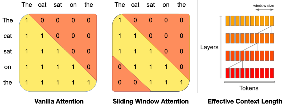
左：vanilla causal attention。中：sliding window（W=3），只保留对角带。右：effective context length —— 堆 k 层之后信息能传播 W·k 个 token

图：Mistral 7B 论文的 SWA 图（Jiang et al. 2023, Fig 1；arXiv:2310.06825）。右图是理解这个机制的关键：单层 SWA 只看 W 个 token，但第 k 层的位置 i 会通过第 k−1 层看到 [i−W, i]，再通过第 k−2 层看到 [i−2W, i]，如此层层递推，信息就以每层 W 的速度向前传播。Mistral 一共 32 层、W=4096，理论感受野可以达到 ≈131K。

Mistral 7B 的具体配置和收益是这样的：\(W = 4096\)；配合 rolling buffer cache，也就是一个固定大小 \(W\) 的环形缓冲，timestep \(i\) 的 K/V 存在槽位 \(i \bmod W\) 里；32K 序列下 cache 内存降低 8 倍且质量无损；FlashAttention/xFormers 侧的相应改动还带来了 16K 长度下 2 倍的加速。

这里有一个值得记住的性质：SWA 是本章唯一一个KV cache 总量存在上界的静态方案。

SWA 的 KV cache 总元素 = 2·h_kv·d_h · 层数 · min(N, W)     ← 与 N 解耦（封顶在 W）

正因为这个性质，它在 Attention 机制 §7 的表里独占一行：不是 \(O(1)\)，但是 \(O(W)\)。

2. attention sink：头几个 token 为什么不能丢¶

如果只保留最近 \(W\) 个 token（也就是纯滑窗、不做重算），perplexity 会直接爆炸。StreamingLLM（arXiv:2309.17453）找到了这背后的原因，而且原因完全来自 softmax 的代数性质，和内容无关。

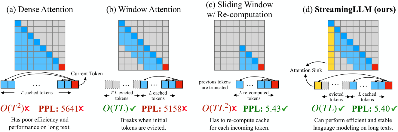
四种方案对比：(a) dense（O(N²)、超出训练长度就崩）(b) window（PPL 5158，崩）(c) sliding with re-computation（PPL 5.43 但 O(N·W²)）(d) StreamingLLM = 4 个 sink + rolling window（PPL 5.40，O(N·W)）

图：StreamingLLM 的核心对照图（Xiao et al. 2023, Fig 1；arXiv:2309.17453）。注意 (b) 和 (d) 的唯一差别就是保留了最前面 4 个 token 的 KV，PPL 从 5158 变成 5.40——差三个数量级。

2.1 根因：softmax 分母恒为正¶

论文 Eq. 1 与那段解释（逐字）：

\[ \mathrm{softmax}(x)_i = \frac{e^{x_i}}{e^{x_1} + \sum_{j=2}^{N} e^{x_j}}, \qquad x_1 \gg x_j \]

"The nature of the SoftMax function prevents all attended tokens from having zero values. This requires aggregating some information from other tokens across all heads in all layers, even if the current embedding has sufficient self-contained information for its prediction. Consequently, the model tends to dump unnecessary attention values to specific tokens."

去掉初始 token 的 KV，会"remove a considerable portion of the denominator in the SoftMax function"，也就是砍掉了分母的一大部分，导致整个 score 分布偏离训练时见过的样子，模型因此崩溃。

为什么恰好是最前面几个 token 起到了这个作用（这是本节第二个关键论据）：

"Due to the sequential nature of autoregressive language modeling, initial tokens are visible to all subsequent tokens, while later tokens are only visible to a limited set of subsequent tokens. As a result, initial tokens are more easily trained to serve as attention sinks."

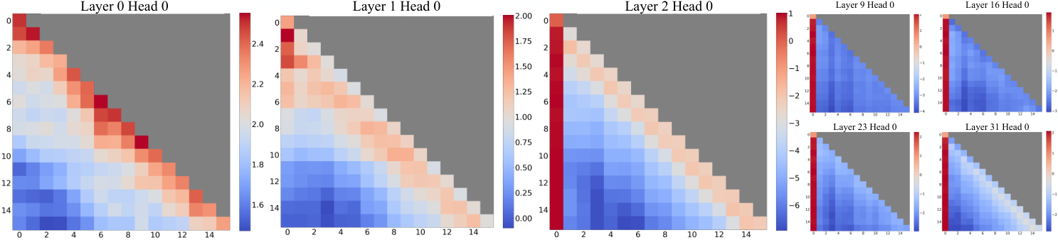
Llama-2-7B 各层的平均 attention logits：第 0–1 层是局部的，**所有更深的层都在 token 0 上出现尖峰**

图：attention sink 现象的直接证据（Xiao et al. 2023, Fig 2；arXiv:2309.17453）。前两层还是正常的局部模式，从第三层开始所有 head 都把大量 attention 倒在第一个 token 上，而这个 token 本身并不携带什么信息，只是充当 softmax 的「泄压阀」。这张图和上一张图放在一起就构成了完整的论证：图 2 说明现象确实存在，图 1 说明去掉它会导致崩溃。

2.2 位置比语义更重要¶

Table 1（Llama-2-13B, PG19）：

Cache config	PPL
`0 + 1024`（纯 window）	5158.07
`4 + 1020`	5.40
`4×"\n" + 1020`（把前 4 个换成换行符）	5.60

这张表说明了一件事：把前 4 个 token 换成毫无语义的换行符，perplexity 基本能恢复，也就是说起作用的是绝对位置，不是内容本身。Table 2 进一步显示 4 个 sink token 就足够：Llama-2-7B 的 PPL 在 0+4096 时是 3359.95，1+4095 时降到 11.88，2+4094 时 10.51，4+4092 时 9.59，8+4088 时 9.54，增益已经很小。

2.3 实现细节：cache 内位置编号¶

原文特别提醒："positions are assigned within the cache, not in the original text"。也就是说，如果 cache 里装着 token [0,1,2,3,6,7,8]，解码第 9 个 token 时用的位置是 [0..7]，不是 [0,1,2,3,6,7,8,9]。

对 RoPE 而言，这意味着key 必须在旋转之前缓存，每一步都要按 cache 内的位置重新旋转。这和 02 §4 里 Dynamic NTK 「必须缓存 pre-RoPE 的 kv」是同一个约束。

def streaming_llm_cache(k_pre_rope, v, n_sink=4, window=1020):
    """k_pre_rope: [B, H, T, D]  未旋转的 key。返回 (k, v, positions)。"""
    k_s, v_s = k_pre_rope[:, :, :n_sink], v[:, :, :n_sink]              # sink：永久保留
    k_w, v_w = k_pre_rope[:, :, -window:], v[:, :, -window:]           # rolling window
    k_cat, v_cat = torch.cat([k_s, k_w], 2), torch.cat([v_s, v_w], 2)
    pos = torch.arange(k_cat.shape[2], device=k_cat.device)            # ← cache 内位置，不是原文位置
    return rope(k_cat, pos), v_cat, pos

其余的实测数字：相对 sliding-window-with-recomputation 有 22.2 倍 的加速；在 Llama-2/MPT/Falcon/Pythia 上可以跑到 4M token；如果预训练时就加一个可学习的 sink token，之后只需要 1 个 sink 就够（普通做法需要 4 个）。这条建议后来被 GPT-OSS 和 DeepSeek-V4 以 learned sink logit 的形式真正落地（02 §5.5）。

3. pattern taxonomy：Longformer 与 BigBird¶

在「按内容动态选择」这一类方法出现之前，静态 pattern 的设计空间已经被 Longformer 和 BigBird 这两篇论文基本穷举过了。

Longformer（arXiv:2004.05150）三种可组合 pattern：

pattern	定义	论文取值
sliding window	query \(i\) attend \([i-w/2, i+w/2]\)	`w = 512`，"therefore using the same amount of computation as RoBERTa"
dilated sliding window	窗口内留间隔 \(d\)	固定 \(d\)、\(w\)、\(\ell\) 层 ⇒ 感受野 \(\ell \cdot d \cdot w\)
global attention	少数预选位置，且对称	`[CLS]` 用于分类；QA 时所有 question token

global pattern 的对称性值得强调，原文写道："a token with a global attention attends to all tokens across the sequence, and all tokens in the sequence attend to it." 因为 global token 的数量与序列长度 \(n\) 无关，总复杂度可以保持在 \(O(n)\)。

BigBird（arXiv:2007.14062）用的是 local + global + random 三者组合，背后的动机来自理论证明：这三种 pattern 组合起来，足以让稀疏 attention 成为序列函数的 universal approximator，并且是 Turing complete 的。HuggingFace 的默认配置是 block_size=64、num_random_blocks=3、window 3 个 block、2 个 global block。序列长度必须能被 block size 整除；如果序列长度低于 1024 token，官方建议直接用 original_full，因为稀疏化在这种规模下不划算。

def bigbird_mask(T, block=64, n_random=3, n_window=3, n_global=2, seed=0):
    """local + global + random 的块级 mask。返回 [T, T] bool。"""
    nb = T // block
    g = torch.Generator().manual_seed(seed)
    blk = torch.zeros(nb, nb, dtype=torch.bool)
    idx = torch.arange(nb)
    for off in range(-(n_window // 2), n_window // 2 + 1):             # local band
        blk |= (idx[None, :] - idx[:, None] == off)
    blk[:, :n_global] = True                                            # global（列：人人都看它）
    blk[:n_global, :] = True                                            # global（行：它看人人）
    for i in range(nb):                                                 # random
        blk[i, torch.randperm(nb, generator=g)[:n_random]] = True
    return blk.repeat_interleave(block, 0).repeat_interleave(block, 1)

这一节的内容之所以重要，是因为后面所有「动态选择」方法都在这个 taxonomy 里保留了静态的骨架：NSA 的 top-\(n=16\) 里就硬编码了 1 个 initial block 加 2 个 local block；MoBA 强制选中当前块；InfLLM-V2 把它写成了显式的并集 \(I = I_{\mathrm{init}} \cup I_{\mathrm{local}} \cup I_{\mathrm{topk}}\)。MoBA 论文更进一步证明了 SWA 和 attention sink 都是自己的特例（04 §7）。可以说，静态 prior 从来没有被真正淘汰，只是被吸收进了动态方法的预算里。

4. 层间交替¶

单层稀疏总会带来一定的信息损失。工业界给出的答案是：让大部分层做稀疏、少数层保持全局，靠这少数全局层兜住长程检索的能力——稀疏由此从算子层面的选择变成了架构层面的设计。

Model	比例	local 形式	window	备注
Gemma 2	1:1（every other layer）	SWA	4096	global 跨度 8192；2B/9B/27B 一致
Gemma 3	5:1，首层是 local	SWA	1024	128K 上下文，只有 ~17% 的层看长程
GPT-OSS	1:1	banded window	128（极小）	per-head learned sink
Llama 4	3:1	chunked（块对角，不是滑窗）	chunk 8192	1/4 层是 NoPE global
Character.AI	~1 global / 6 层	——	——	+ cross-layer KV sharing + MQA，报 ~20× cache 减少

Gemma 2 的原文是："We alternate between a local sliding window attention and global attention in every other layer." Gemma 3 的原文则是："5:1 interleaving of local/global layers … a pattern of 5 local layers for every global layer, starting with a local layer as the first layer of the model."

Gemma 3 有两个很实用的消融结论：Fig 3 显示 local:global 的比例对 perplexity 的影响 "minimal impact"；Fig 4 显示窗口大小 "can be reduced significantly without impacting perplexity"（Gemma 2 的 Table 10 给出了更直接的数字：window 取 4096/2048/1024 时 PPL 分别是 1.63/1.63/1.64，几乎没有差别）。也就是说，质量对这两个旋钮都不敏感，而内存开销对它们却极其敏感：在 32K 上下文下，全局层全用 global attention 的 cache 占到模型权重的 60%，而换成 1:3 + sw=1024 之后能降到 不到 15%。这几乎是「免费」拿到的 8 倍内存节省。

Llama 4 的 chunked attention¶

⚠️ 一个流传很广的误解是把 Llama 4 的 local attention 当作 sliding window，值得单独澄清：它实际上是 chunked attention。官方 llama-models 参考实现如下：

def create_chunked_attention_mask(seq_len, attention_chunk_size, device):
    block_pos = torch.abs(
        (torch.arange(seq_len).unsqueeze(0) // attention_chunk_size)
        - (torch.arange(seq_len).unsqueeze(1) // attention_chunk_size))
    token_pos = torch.arange(seq_len).unsqueeze(0) - torch.arange(seq_len).unsqueeze(1)
    mask = (block_pos == 0) & (token_pos <= 0)          # 必须同块 + causal
    return mask

block_pos == 0 意味着 query 和 key 必须落在同一个 chunk 里，这实际上是一个块对角 causal mask：token 0..K 之间互相可见，K..2K 之间互相可见，但跨块完全不通。而滑窗是每个 query 都有自己平移的窗口，两者的结构并不相同。

这带来的后果是：chunked attention 不能像堆叠 SWA 那样跨块传播信息（§1 右图描述的那个机制在这里不成立），这正是 Llama 4 必须搭配 NoPE 全 attention 层的原因。它的 attention_chunk_size 取值是 8192。vLLM 把这两种模式分别建模成 ChunkedLocalAttentionSpec 和 FullAttentionSpec。

Meta 的 iRoPE 说法：

"A key innovation in the Llama 4 architecture is the use of interleaved attention layers without positional embeddings. Additionally, we employ inference time temperature scaling of attention to enhance length generalization. We call this the iRoPE architecture, where 'i' stands for 'interleaved'."

具体的 config 是：no_rope_layers: [1,1,1,0, 1,1,1,0, …]（48 层，每 4 层里有 1 层是 NoPE）；attn_temperature_tuning: true、attn_scale: 0.1、floor_scale: 8192。这里 temperature scaling 只用在 NoPE 层上，HF 的文档明确写道："applied in the NoPE layers, but not in the RoPE ones as these attend to shorter sub-sequences"。Scout 在预训练和后训练阶段都用 256K，官方声称支持到 10M。

Llama 4 的分工：
  RoPE + chunked local (8192)  →  短程精确顺序，cache 封顶、算力省
  NoPE + full global           →  跨全上下文检索，不会因超出训练长度而旋转角失配

5. 推理期动态稀疏及其局限¶

这一类方法不改训练，只在推理时按内容临时做选择，代表性的有三类：

Quest（arXiv:2406.10774，ICML 2024）做的是 query-aware page selection，用在 decode 阶段。它给每个 page 维护 key 的 channel-wise min \(m_i\) 和 max \(M_i\)；给定 query \(Q\)，逐通道算出上界 \(U_i = \max(Q_i m_i,\ Q_i M_i)\)，那么 \(\sum_i U_i\) 就是该 page 内最高 attention score 的上界。按这个上界选 top-\(K\) page，就不容易漏掉真正重要的 token。

def quest_page_scores(q, k, page=16):
    """q: [B,H,1,D] (decode)。k: [B,H,N,D]。返回每个 page 的上界打分 [B,H,N/page]。"""
    kp = k.unflatten(2, (-1, page))                    # [B,H,NP,page,D]
    m, M = kp.amin(3), kp.amax(3)                      # channel-wise min / max，每 page 各 D 维
    return torch.maximum(q.transpose(2, 3) * m, q.transpose(2, 3) * M).sum(-1)

算一下代价：page 大小为 \(S\)、上下文长度为 \(N\)，选 top-\(K\) 时实际要读的 cache 比例是 \(1/S + KS/N\)；取 \(S=16\)、64K 上下文、top-4K，能拿到 8 倍的减少。

MInference 1.0（arXiv:2407.02490，NeurIPS 2024）走的是 training-free 路线，但只加速 prefill。它定义了三种 head 级 pattern：

pattern	结构	索引怎么来
A-shape	global prefix + local 对角带（≈StreamingLLM）	静态；参考配置 1024 global + 4096 local
Vertical-Slash	少数特定列 + 斜线状对角	动态：用最后 `last_q` 个 query 对全部 K 估计
Block-Sparse	散落但空间聚集的稠密块	动态：Q/K 按 64 分块 mean-pool，块级打分

每个 head 归属哪种 pattern，由离线的 Kernel-Aware Sparse Pattern Search 决定，具体索引则在线上构建。这样能省下约 95% 的 attention FLOPs，在 A100 上 prefill 最高能加速 10 倍。

H2O / SnapKV / SepLLM 走的是另一条路，即 KV eviction：按累积的 attention 质量丢弃「不重要」的 token。

局限的三个原因¶

原因一是阶段受限。 MInference 只能加速 prefill，Quest 只能加速 decode，两者互相覆盖不到对方。MoBA 在评测时也承认了这一点："MoBA is used for prefill only, while we switch to full attention during generation"。而 Attention 机制 §1 那个式子已经说明，真正花钱的地方是 decode，仅加速 prefill 解决不了核心问题。

原因二更根本，是 GQA 下「算力稀疏不等于访存稀疏」这一点。 这是 NSA 论文对 Quest 的核心批评，也是理解整条 sparse 路线走向的关键：

GQA，一组 g 个 query head 共享一份 KV。
每个 head 独立选自己的 top-k pages
  ⇒ 实际必须从 HBM 搬的字节 = 组内 g 个 head 选择集合的【并集】
  ⇒ 计算量降了 k/N，但访存量降得远少于 k/N
  ⇒ 而 decode 是 memory-bound（[README] §1）⇒ 加速远不如账面

NSA 给出的解法是 Eq. 10：把组内所有 head 的打分加起来，强制一整组共用一份 block 列表（04 §3）。DSA 的解法更极端：用 MLA 的 MQA mode，让一个 latent 被所有 head 共享，这样 per-query 的 token 级选择就自动满足访存稀疏了（05 §3）。

原因三是 post-hoc 剪枝存在质量天花板。 NSA 引用的一个量化论据是：top-20% 的 attention 只覆盖了 70% 的 attention 质量（Chen et al. 2024b），所以 dense 预训练模型里的 retrieval head 经不起事后剪枝。NSA 还试过「先用 1000 步 full attention 冷启动、再切换到启发式 blockwise 选择」这种折中方案，结果仍然不如原生训练的 NSA。

NSA 的 LongBench 对照（所有 sparse baseline 都给 2560 个激活 token 以求公平）：

方法	LongBench avg
NSA（原生训练）	0.469
Full Attention	0.437
Exact-Top	0.423
Quest	0.392
InfLLM	0.383
H2O	0.303

值得注意的是，NSA 甚至超过了 Full Attention 的表现。这个反直觉的结果正是 04 的起点：稀疏不只是用来省钱的手段，训练时带着稀疏约束本身，可能还是一种有益的归纳偏置。

6. 小结¶

类别	代表	每 token cache	加速哪个阶段	天花板
SWA	Mistral、Gemma local、GPT-OSS local	封顶 \(O(W)\)	两个都	单层感受野只有 \(W\)，靠堆层传播（chunked 连这个都没有）
window + sink	StreamingLLM	封顶	decode（streaming）	只能流式，不能真正检索长上下文
local+global(+random)	Longformer、BigBird	\(O(N)\) 但常数小	两个都	pattern 与内容无关
层间交替	Gemma 2/3、GPT-OSS、Llama 4	少数层随 \(N\) 增长	两个都	实际最成功的静态方案；全局层仍是 \(O(N^2)\)
推理期动态	Quest、MInference、H2O	全量	只有一个阶段	阶段受限 + GQA 访存不稀疏 + post-hoc 质量损失

静态方案，尤其是层间交替这一类，在工业界非常成功且几乎是免费的，Gemma 3、GPT-OSS、Llama 4 都靠它撑住了 128K 的上下文。它的上限在于「pattern 不看内容」。推理期动态方案想要看内容却又不改训练，结果被 GQA 的访存约束和 post-hoc 的质量天花板一起夹住，两头都没能做到最好。

这两个约束合起来指向同一个结论：要么让选择变成块级且组内一致（NSA/MoBA 的做法），要么让 KV entry 被所有 head 共享（DSA 的做法），而且最好从一开始就原生训练，而不是事后打补丁。这正是下一篇要展开的内容。

下一篇：04 · sparse 路线（二）：可训练稀疏。2025 年 2 月，NSA 和 MoBA 相隔三天出现，用两种完全不同的哲学回答了同一个问题：怎么让稀疏 attention 从训练第一步就存在。