03 · Sequence Parallelism:AG/RS 替换 all-reduce
SP 出自 Korthikanti et al. 2022 年发表的 Reducing Activation Recomputation in Large Transformer Models(arXiv:2205.05198,也就是提出 Megatron-SP 和 selective activation recomputation 的那篇论文)。它要解决的问题很直接:TP 省下了权重和算力,但没有省下 activation 的显存——TP 区外的 LayerNorm、dropout、residual 输入,在每张卡上都是完整复制的 \([s, b, h]\)。SP 的做法是把这些也按 sequence 维切到 TP 各卡上,让 activation 显存随着 TP 线性下降。
1. TP 区外的 activation 被完整复制
回顾一下 02 里讲到的内容:一个 layer 里激活的状态是这样的
[LN] → [attention: col→row, all-reduce] → [dropout+residual] → [LN] → [MLP: col→row, all-reduce] → [dropout+residual]
 ↑复制              ↑区内切开                      ↑复制            ↑复制         ↑区内切开                  ↑复制
标注「复制」的地方——也就是 LayerNorm 的输入/输出、dropout、residual——在 TP 各卡上是逐元素相同的完整 \([s, b, h]\)。以 TP=8 为例,这相当于把同一份 activation 存了 8 遍。而这些 activation 又都要保留到 backward 才能释放,是显存开销的大头。
这里有一个关键的观察:LayerNorm、dropout、residual add 这些操作,都是沿 hidden 维独立、沿 sequence 维也独立的操作——element-wise 计算,或者是沿 hidden 维做的归一化,跟别的 token 完全没有关系。所以完全可以把 sequence 维 \(s\) 切成 \(s/\mathrm{TP}\),每张卡只处理 \([s/\mathrm{TP}, b, h]\),各自算各自的,不需要任何通信。
2. 解法:all-reduce = reduce-scatter + all-gather,拆开来用
核心恒等式:
从通信量上看,all-reduce 大约是 2 倍数据量,而 RS 和 AG 各自约是 1 倍数据量。所以把一次 all-reduce 拆成「出口的 RS 加入口的 AG」,总字节数是不变的,但中间会多出一段「activation 按 seq 切开」的状态,这一段就是 SP 区,activation 在这里只需要存 \(1/\mathrm{TP}\)。
flowchart LR
    subgraph SP1["SP 区 (seq 切开 [s/TP,b,h])"]
        LN1["LayerNorm\n(本地, 按 s/TP)"]
    end
    LN1 -->|"g_sp = all-gather (seq)\n凑齐 [s,b,h]"| TP1
    subgraph TP1["TP 区 (hidden 切开)"]
        ATT["attention col→row GEMM"]
    end
    ATT -->|"f_sp = reduce-scatter (seq)\n规约+切回 [s/TP,b,h]"| SP2
    subgraph SP2["SP 区"]
        DR["dropout+residual\n(本地, 按 s/TP)"]
    end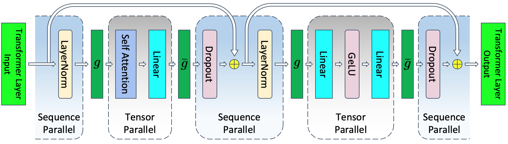
图:TP+SP 合并后的一整个 transformer layer。SP 区(LayerNorm、dropout、residual)按 sequence 维切成
[s/TP,b,h];进 TP 区用g(forward all-gather,凑齐s),出 TP 区用ḡ(forward reduce-scatter,规约+切回s/TP)。g与ḡ互为共轭:g= forward all-gather / backward reduce-scatter,ḡ= forward reduce-scatter / backward all-gather。注意这里论文的g/ḡ记号与 Megatron 源码里替换掉的f/g对应关系(见下表)。(Korthikanti et al. 2022, Fig 5;arXiv:2205.05198)
对照 README 里定义的 f/g:SP 把 f 实现成 all-gather(forward)加 reduce-scatter(backward),把 g 实现成 reduce-scatter(forward)加 all-gather(backward)。它们仍然互为共轭:
| 算子 | forward | backward | 代码 |
|---|---|---|---|
进 TP 区(替代 f) |
all-gather (seq) | reduce-scatter (seq) | _GatherFromSequenceParallelRegion mappings.py:L296 |
出 TP 区(替代 g) |
reduce-scatter (seq) | all-gather (seq) | _ReduceScatterToSequenceParallelRegion mappings.py:L351 |
3. AG/RS 的代码落点
SP 的这两半通信,分别落在 01 已经讲过的两个地方:
-
进入 TP 区的 all-gather:不在 module 层,而是在
LinearWithGradAccumulationAndAsyncCommunication.forward内部(layers.py:L499–L505)。column-parallel 收到的输入是 \([s/\mathrm{TP}, b, h]\),GEMM 之前会先 all-gather 成 \([s, b, h]\)。backward 时(layers.py:L569–L578)对 dgrad 做 reduce-scatter,输出直接就是 \([s/\mathrm{TP}, b, h]\)。 -
离开 TP 区的 reduce-scatter:在
RowParallelLinear.forward(layers.py:L1352):它一步就完成了两件事——「把 row 的部分和规约起来」和「按 seq 切回去」,输出的 \([s/\mathrm{TP}, b, h]\) 正好可以直接喂给下一段 SP 区的 dropout+residual。elif self.sequence_parallel: output_ = reduce_scatter_to_sequence_parallel_region(output_parallel, group=self.tp_group)
_split_along_first_dim / _gather_along_first_dim / _reduce_scatter_along_first_dim(mappings.py:56/114/155)都作用在第 0 维(也就是 sequence 维)上,这也是「sequence parallel」这个名字的由来。
4. 完整 TP+SP 数据流(一个 layer)
[s/TP,b,h] ──AG(seq)──► [s,b,h] ──QKV(col)──► attn(本地 head) ──proj(row)──► 部分和 ──RS(seq)──► [s/TP,b,h]
   SP:LN                  TP region                                                         SP:dropout+resid
[s/TP,b,h] ──AG(seq)──► [s,b,h] ──fc1(col)──► act ──fc2(row)──► 部分和 ──RS(seq)──► [s/TP,b,h]
   SP:LN                  TP region                                          SP:dropout+resid
- 每个 layer:forward 需要 2 次 AG 加 2 次 RS,用来替代纯 TP 下的 2 次 all-reduce,通信字节数和纯 TP 是相同的。
- activation 显存:LayerNorm/dropout/residual 的 activation 从 \([s, b, h]\) 降到 \([s/\mathrm{TP}, b, h]\),随着 TP 线性下降,这是 SP 存在的唯一目的。
- backward 会自动镜像:AG 和 RS 对调(见上表),这是 autograd 免费给出的,不需要额外实现。
5. sp2hp / hp2sp:另一种「seq↔hidden」切换(mappings.py:562/591)
在某些场景下(比如 MoE 的 token 在 TP 维上分布、或者某些 fused kernel),需要在这两种切分方式之间来回转换:
all_to_all_sp2hp: [num_tokens/TP, H]  →  [num_tokens, H/TP]   (seq-切 → hidden-切)
all_to_all_hp2sp: [num_tokens, H/TP]  →  [num_tokens/TP, H]   (hidden-切 → seq-切)
实现方式是 torch.split 加 all_to_all 加 cat(mappings.py:578/610):用一次 all-to-all,把「按 seq 切」转成「按 hidden 切」。这在 SP 和某些 TP-fused 算子(或者 Ulysses 风格的 CP,见 CP)衔接的地方会用到。底层都是 _AllToAll(mappings.py:L420),它的 backward 是把 split 方向对调之后的 all-to-all,和 MoE 的 dispatch 是同构的。
6. SP 的工程收益与代价
| 维度 | 纯 TP | TP + SP |
|---|---|---|
| 权重显存 | \(1/\mathrm{TP}\) | \(1/\mathrm{TP}\) |
| activation(区内) | \(1/\mathrm{TP}\) | \(1/\mathrm{TP}\) |
| activation(区外 LN/dropout/resid) | ×1(复制) | \(1/\mathrm{TP}\) |
| forward 通信 | 2× all-reduce | 2× AG + 2× RS(同字节数) |
| 通信可 overlap 性 | 较难 | 更好(AG/RS 颗粒更细,易和 GEMM 流水) |
| 实现复杂度 | 低 | 中(要管 seq 维 split、和 CP/PP 的 seq 维耦合) |
SP 几乎是免费的:通信量不变,显存却显著下降,所以在 Megatron 里只要开了 TP,基本都会顺手把 SP(
sequence_parallel=True)也开上。唯一的约束是 \(s\) 要能被 TP 整除,并且要和同样切 seq 维的 CP 协调好切分的先后顺序。
讲完 SP 的原理和数据流,接下来自然要问:这些通信在工程上是怎么被藏进计算里的?CUDA_DEVICE_MAX_CONNECTIONS=1 到底在起什么作用、async all-reduce/RS 怎么和 wgrad 做 overlap、tp_comm_overlap(也就是 userbuffers)又是怎么把 AG/RS 拆进 GEMM 的 tile 里做细粒度流水的,这些都在04 · TP/SP 的通信-计算 overlap 与工程优化里。